Xenium Prime 5K (codeword)

This notebook demonstrates essential steps for analyzing spatial codeword (exon/junction probes) usage in Xenium Prime 5K data, using the 10x Genomics Xenium Prime 5K Mouse Brain Coronal dataset as an example.

1. Load codeword-level quantification as binned spatial data.

2. Run FFT-accelerated spatial variability tests with SplisosmFFT.

3. Compare results across spatial resolutions and with SplisosmNP.

For differential usage testing with SplisosmFFT, see the Visium HD FFPE (probe) Part II tutorial. Additionally, a SplisosmNP-based workflow using cell-segmentation results is available in the Single-cell segmented data (Xenium Prime 5K) tutorial.

Estimated runtime: ~5 min.

Preliminary notes

For Xenium Prime 5K datasets, each gene is profiled by multiple codewords (i.e., exon/junction probe sets). This notebook uses the same Xenium dataset as presented in the SPLISOSM paper and as in the Single-cell segmented data tutorial.

• The dataset can be downloaded from 10x Genomics here

• Probe set (5K Mouse Pan Tissue and Pathways Panel) information is available here.

After downloading Xenium analysis outputs, we reran the Xenium Ranger v3.1.0 relabel pipeline to get codeword transcript counts. Due to Xenium output data structure changes, if you encounter issues, consider re-running the Xenium Ranger (v3.1.0+) relabel pipeline as well. See 10x documentation for guidance.

Imports

from __future__ import annotations

from pathlib import Path
import warnings

import numpy as np
import pandas as pd
import matplotlib.pyplot as plt
from scipy.stats import spearmanr

import spatialdata as sd
import spatialdata_plot  # Registers plotting accessors
from spatialdata import rasterize_bins

from splisosm import SplisosmFFT, SplisosmNP
from splisosm.utils import counts_to_ratios
from splisosm.io import load_xenium_codeword

warnings.filterwarnings('ignore', category=FutureWarning)
plt.rcParams['figure.dpi'] = 120
plt.rcParams['figure.figsize'] = (6, 4)

Configure paths and core parameters

# Required: Xenium Ranger output directory (either the `outs` dir itself or its parent)
xenium_prime_outs = Path('/path/to/xenium_prime_5k/outs')

# Optional cache path
sdata_zarr = xenium_prime_outs / 'sdata_codeword.filtered.zarr'

# Optional probe annotation BED for visualization
bed_file = Path("/path/to/xenium_5k_probe_locations.bed")
# Optional gene annotation GTF for gene symbol mapping
gtf_file = Path("/path/to/mm10/gencode.vM23.annotation.gtf.gz")

# Resolutions (um) to materialize
spatial_resolutions = [8.0, 16.0]

# Primary analysis table / bins
test_table = 'square_016um'
test_bins_element = 'square_016um_bins'

# Feature grouping and filters
group_iso_by = 'gene_symbol'
gene_name_col = 'gene_symbol'
min_counts = 10
min_bin_pct = 0.0

# Xenium transcript filter
quality_threshold = 20.0

Load codeword-level SpatialData

We use splisosm.io.load_xenium_codeword to read transcripts.zarr.zip directly and optionally bin transcripts into square units of fixed resolutions.

%%time
if sdata_zarr.exists():
    print('Loading cached SpatialData...')
    sdata = sd.read_zarr(sdata_zarr)
else:
    print('Building Xenium codeword SpatialData from transcript chunks...')
    sdata = load_xenium_codeword(
        path=xenium_prime_outs,
        spatial_resolutions=spatial_resolutions,
        quality_threshold=quality_threshold,
        n_jobs=-1,
        chunk_batch_size=64,
        counts_layer_name='counts',
        build_cell_codeword_table=True,
        create_square_shapes=True,
        show_progress=True,
    )
    # Optional: cache for faster reruns
    # sdata.write(sdata_zarr)

sdata

Building Xenium codeword SpatialData from transcript chunks...

/Users/jysumac/miniforge3/envs/splisosm_dev/lib/python3.12/functools.py:912: ImplicitModificationWarning: Transforming to str index.
  return dispatch(args[0].__class__)(*args, **kw)

WARNING  The `feature_key` column feature_name is categorical with unknown categories. Please ensure the categories
         are known before calling `PointsModel.parse()` to avoid significant performance implications due to the   
         need for dask to compute the categories. If you did not use PointsModel.parse() explicitly in your code   
         (e.g. this message is coming from a reader in `spatialdata_io`), please report this finding.              

CPU times: user 2min 1s, sys: 28.2 s, total: 2min 29s
Wall time: 1min 7s

SpatialData object
├── Images
│     └── 'morphology_focus': DataTree[cyx] (4, 23912, 34154), (4, 11956, 17077), (4, 5978, 8538), (4, 2989, 4269), (4, 1494, 2134)
├── Labels
│     ├── 'cell_labels': DataTree[yx] (23912, 34154), (11956, 17077), (5978, 8538), (2989, 4269), (1494, 2134)
│     └── 'nucleus_labels': DataTree[yx] (23912, 34154), (11956, 17077), (5978, 8538), (2989, 4269), (1494, 2134)
├── Points
│     └── 'transcripts': DataFrame with shape: (<Delayed>, 13) (3D points)
├── Shapes
│     ├── 'cell_boundaries': GeoDataFrame shape: (63173, 1) (2D shapes)
│     ├── 'nucleus_boundaries': GeoDataFrame shape: (63036, 1) (2D shapes)
│     ├── 'square_008um_bins': GeoDataFrame shape: (576580, 1) (2D shapes)
│     └── 'square_016um_bins': GeoDataFrame shape: (144372, 1) (2D shapes)
└── Tables
      ├── 'square_008um': AnnData (576580, 11163)
      ├── 'square_016um': AnnData (144372, 11163)
      ├── 'table': AnnData (63173, 5006)
      └── 'table_codeword': AnnData (63173, 11163)
with coordinate systems:
    ▸ 'global', with elements:
        morphology_focus (Images), cell_labels (Labels), nucleus_labels (Labels), transcripts (Points), cell_boundaries (Shapes), nucleus_boundaries (Shapes), square_008um_bins (Shapes), square_016um_bins (Shapes)

In Xenium Prime 5K datasets, each codeword corresponds to a specific probe set for a gene. Here, we will focus on the codeword-level counts tables:

• sdata.tables['table_codeword'] contains cell-by-codeword counts aggregated to segmented cells.

• sdata.tables['square_*um'] contains bin-by-codeword counts aggregated at various resolutions.

def summarize_table(adata):
    X = adata.layers['counts'] if 'counts' in adata.layers else adata.X
    if hasattr(X, 'nnz'):
        nnz = int(X.nnz)
        total = int(X.shape[0] * X.shape[1])
        density = nnz / total if total else np.nan
    else:
        arr = np.asarray(X)
        nnz = int(np.count_nonzero(arr))
        total = int(arr.size)
        density = nnz / total if total else np.nan
    return {
        'n_features': int(adata.n_vars),
        'n_bins': int(adata.n_obs),
        'count_mtx_density': density,
    }

rows = []
for key in sorted(sdata.tables.keys()):
    rows.append({'table': key, **summarize_table(sdata.tables[key])})

table_summary = pd.DataFrame(rows).sort_values('table')
table_summary

	table	n_features	n_bins	count_mtx_density
0	square_008um	11163	576580	0.018701
1	square_016um	11163	144372	0.058018
2	table	5006	63173	0.139117
3	table_codeword	11163	63173	0.077513

Note that only data with regular spacing (e.g., square_016um) are suitable for FFT-based spatial variability analysis. For illustration purposes, we will run analysis on the square_016um table and use the shape square_016um_bins (i.e., spatial grid with 16 × 16 µm bins) for rasterization.

print('Tables:', sorted(sdata.tables.keys()))
print('Shapes:', sorted(getattr(sdata, 'shapes', {}).keys()))
print('Images:', sorted(getattr(sdata, 'images', {}).keys()))

if test_table not in sdata.tables:
    raise ValueError(f'{test_table} is not available. Choose from: {sorted(sdata.tables.keys())}')
if test_bins_element not in sdata.shapes:
    raise ValueError(f'{test_bins_element} is not available. Choose from: {sorted(sdata.shapes.keys())}')

adata_test = sdata.tables[test_table]
if group_iso_by not in adata_test.var.columns:
    raise ValueError(f'{group_iso_by} not found in {test_table}.var columns')

print(f'Using table={test_table}, bins={test_bins_element}')
print(f'Grouping column={group_iso_by}, display names={gene_name_col}')

Tables: ['square_008um', 'square_016um', 'table', 'table_codeword']
Shapes: ['cell_boundaries', 'nucleus_boundaries', 'square_008um_bins', 'square_016um_bins']
Images: ['morphology_focus']
Using table=square_016um, bins=square_016um_bins
Grouping column=gene_symbol, display names=gene_symbol

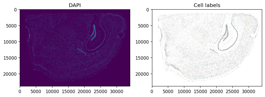
Morphology and segmentation preview

%%time
axes = plt.subplots(1, 2, figsize=(10, 5))[1].flatten()
sdata.pl.render_images(f"morphology_focus", channel='DAPI').pl.show(
    coordinate_systems=f"global",
    ax=axes[0], title="DAPI", colorbar=False
)
sdata.pl.render_labels(f"cell_labels").pl.show(
    coordinate_systems=f"global",
    ax=axes[1], title="Cell labels"
)

/Users/jysumac/miniforge3/envs/splisosm_dev/lib/python3.12/site-packages/pims/tiff_stack.py:131: UserWarning: <tifffile.TiffPage 0 @16> reading array from closed file
  data = t.asarray()

CPU times: user 3min 26s, sys: 13.5 s, total: 3min 39s
Wall time: 32.6 s

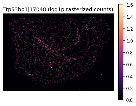
Rasterize bins and visualize one codeword

%%time
# rasterize_bins() expects a CSC matrix for best compatibility
adata_plot = sdata.tables[test_table]
adata_plot.X = adata_plot.layers['counts']
if hasattr(adata_plot.X, 'tocsc') and getattr(adata_plot.X, 'format', None) != 'csc':
    adata_plot.X = adata_plot.X.tocsc()

raster_key = f'rasterized_{test_table}'
sdata[raster_key] = rasterize_bins(
    sdata,
    bins=test_bins_element,
    table_name=test_table,
    col_key='array_col',
    row_key='array_row',
)
print('Created:', raster_key)

Created: rasterized_square_016um
CPU times: user 776 ms, sys: 174 ms, total: 950 ms
Wall time: 956 ms

%%time
feature_name = 'Trp53bp1|17048' # Trp53bp1
img = np.asarray(sdata[f'rasterized_{test_table}'].sel(c=feature_name).values).squeeze()

fig, ax = plt.subplots(figsize=(5, 4))
im = ax.imshow(np.log1p(img), cmap='magma')
ax.set_title(f'{feature_name} (log1p rasterized counts)')
ax.axis('off')
fig.colorbar(im, ax=ax, fraction=0.046, pad=0.04)
plt.show()

CPU times: user 51.1 ms, sys: 7.33 ms, total: 58.4 ms
Wall time: 67.3 ms

Spatial variability testing with SplisosmFFT

model = SplisosmFFT(neighbor_degree=1, rho=0.99)
model.setup_data(
    sdata=sdata,
    bins=test_bins_element,
    table_name=test_table,
    col_key='array_col',
    row_key='array_row',
    layer='counts',
    group_iso_by=group_iso_by,
    gene_names=gene_name_col,
    min_counts=min_counts,
    min_bin_pct=min_bin_pct,
    filter_single_iso_genes=True
)
model

=== SplisosmFFT
- Number of genes: 4972
- Number of spots: 144372
- Number of spots after rasterization: 144372
- Number of covariates: 0
- Average isoforms per gene: 2.1
=== Model configurations
- Neighborhood degree: 1
- Spatial autocorrelation rho: 0.99
=== Test results
- Spatial variability: N/A
- Differential usage: N/A

Before running the test, we can again check gene-level summaries to confirm that Xenium Prime 5K data contains multiple codewords per gene.

%%time
gene_meta = model.extract_feature_summary(level='gene')
gene_meta.sort_values('perplexity', ascending=False).head(5)

Genes: 100%|██████████| 4972/4972 [00:04<00:00, 1140.05it/s]

CPU times: user 4.27 s, sys: 548 ms, total: 4.82 s
Wall time: 4.84 s

	n_isos	perplexity	pct_bin_on	count_avg	count_std	major_ratio_avg
gene
Gnao1	4	3.979105	0.616671	4.027173	5.066839	0.292012
Apob	4	3.952770	0.001385	0.002016	0.141543	0.288660
Gja1	4	3.929913	0.375149	1.565989	3.772387	0.333883
Acox1	4	3.921495	0.459334	1.000139	1.440174	0.301513
Ghr	4	3.909349	0.041268	0.045805	0.233034	0.308937

%%time
model.test_spatial_variability(
    method='hsic-ir',
    ratio_transformation='none',
    n_jobs=-1,
    print_progress=True,
)
sv_res_fft = model.get_formatted_test_results(
    'sv', with_gene_summary=True
).sort_values('pvalue_adj')

SV [hsic-ir]: 100%|██████████| 331/331 [00:14<00:00, 22.16it/s]

CPU times: user 1min 11s, sys: 13.4 s, total: 1min 24s
Wall time: 15.6 s

sig_001 = int((sv_res_fft['pvalue_adj'] < 0.01).sum())
print(
    'Spatially variable genes (FDR < 0.01): '
    f'{sig_001} out of {sv_res_fft.shape[0]} total genes'
)
sv_res_fft.head(5)

Spatially variable genes (FDR < 0.01): 2158 out of 4972 total genes

	gene	statistic	pvalue	pvalue_adj	n_isos	perplexity	pct_bin_on	count_avg	count_std	major_ratio_avg
1230	Pja1	2.192375e-06	0.0	0.0	2	1.980112	0.230211	0.328949	0.703162	0.570571
643	Fap	1.540108e-07	0.0	0.0	3	2.600355	0.011837	0.013257	0.130763	0.509404
2978	Syne1	4.315414e-06	0.0	0.0	2	1.999256	0.303037	0.593363	1.207081	0.513640
673	Cyp26b1	1.980515e-07	0.0	0.0	2	1.409796	0.022560	0.038865	0.374784	0.891463
3648	Vamp2	2.441610e-06	0.0	0.0	2	1.995571	0.602575	3.061141	3.648642	0.533281

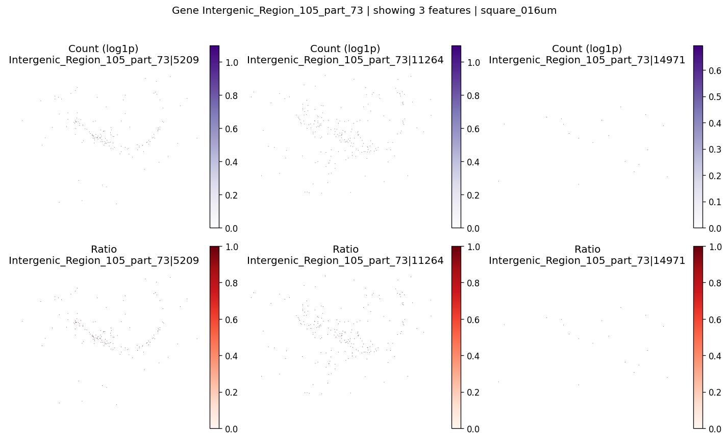
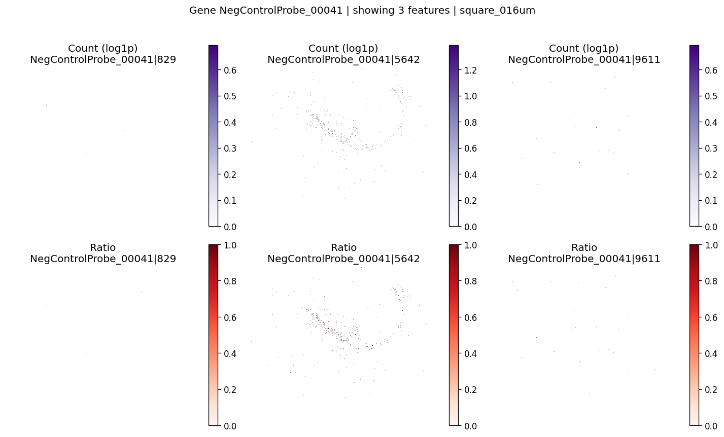
We can use negative control probes to estimate false positive rates due to technical noise (e.g., probe malfunction or non-specific hybridization).

ctrl_genes = (
    sv_res_fft['gene'].str.startswith('NegControlProbe') |
    sv_res_fft['gene'].str.startswith('Intergenic')
)
sig_001_ctrl = int((sv_res_fft.loc[ctrl_genes, 'pvalue_adj'] < 0.01).sum())
print(
    'Spatially variable negative control genes (FDR < 0.01): '
    f'{sig_001_ctrl} out of {sv_res_fft.loc[ctrl_genes].shape[0]} total control genes'
)
sv_res_fft.loc[ctrl_genes].sort_values('pvalue_adj').head(5)

Spatially variable negative control genes (FDR < 0.01): 9 out of 57 total control genes

	gene	statistic	pvalue	pvalue_adj	n_isos	perplexity	pct_bin_on	count_avg	count_std	major_ratio_avg
2475	Intergenic_Region_105_part_73	2.199321e-08	5.841736e-17	4.277630e-16	3	2.321053	0.002625	0.002701	0.053352	0.551282
463	NegControlProbe_00041	5.502025e-09	1.514442e-07	6.413802e-07	2	1.266769	0.002944	0.003055	0.057399	0.936508
731	NegControlProbe_00003	5.328555e-09	2.520976e-07	1.040190e-06	3	1.655403	0.001365	0.001365	0.036914	0.857868
1042	Intergenic_Region_10757_part_30	8.702548e-09	7.845542e-05	2.456425e-04	3	2.391157	0.001081	0.001081	0.032854	0.608974
1105	NegControlProbe_00014	1.269646e-08	2.300467e-04	6.740084e-04	3	2.061472	0.002092	0.002092	0.045689	0.754967

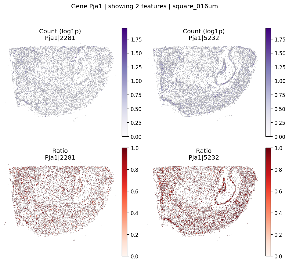
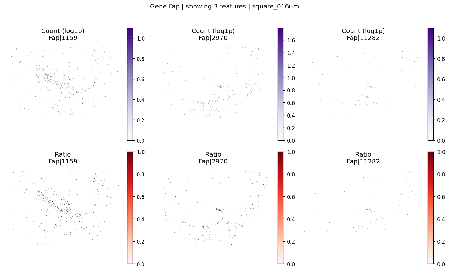
Visualize selected significant genes

def ensure_rasterized(sdata, bin_table: str, bin_element: str, layer: str = 'counts'):
    raster_key = f'rasterized_{bin_table}_{layer}'
    if raster_key in sdata.images:
        return raster_key

    adata = sdata.tables[bin_table]
    adata.X = adata.layers[layer]
    if hasattr(adata.X, 'tocsc') and getattr(adata.X, 'format', None) != 'csc':
        adata.X = adata.X.tocsc()

    sdata[raster_key] = rasterize_bins(
        sdata,
        bins=bin_element,
        table_name=bin_table,
        col_key='array_col',
        row_key='array_row',
    )
    return raster_key

def plot_gene_codeword_maps(
    sdata,
    bin_table: str,
    bin_element: str,
    gene_id: str,
    var_meta: pd.DataFrame | None = None,
    group_col: str = 'gene_symbol',
    max_features: int = 4,
    hide_zero_count: bool = True,
    hide_zero_ratio: bool = True,
):
    adata = sdata.tables[bin_table]
    if var_meta is None:
        var_meta = adata.var.copy()

    if group_col not in var_meta.columns:
        raise ValueError(f"'{group_col}' not found in var metadata columns")

    feature_names = var_meta.index[var_meta[group_col].astype(str) == str(gene_id)].tolist()
    if len(feature_names) == 0:
        raise ValueError(f"No features found for gene '{gene_id}'")

    feature_names = feature_names[: min(len(feature_names), max_features)]

    raster_key = ensure_rasterized(sdata, bin_table=bin_table, bin_element=bin_element)
    data = sdata[raster_key].sel(c=feature_names).values
    counts_cube = np.moveaxis(np.asarray(data, dtype=float), 0, -1)

    counts_flat = counts_cube.reshape(-1, counts_cube.shape[-1])
    ratios_flat = counts_to_ratios(counts_flat, transformation='none', nan_filling='none')
    ratios_cube = ratios_flat.numpy().reshape(counts_cube.shape)

    n_feat = counts_cube.shape[-1]
    fig, axes = plt.subplots(2, n_feat, figsize=(4 * n_feat, 7), squeeze=False)

    vmax_ratio = np.nanpercentile(ratios_cube, 99) if np.isfinite(ratios_cube).any() else 1.0

    for i, feature in enumerate(feature_names):
        c = counts_cube[:, :, i]
        r = ratios_cube[:, :, i]

        if hide_zero_count:
            c = np.where(c == 0, np.nan, c)
        if hide_zero_ratio:
            r = np.where(r == 0, np.nan, r)

        im0 = axes[0, i].imshow(np.log1p(c), cmap='Purples', vmin=0.0)
        axes[0, i].set_title(f'Count (log1p)\n{feature}')
        axes[0, i].axis('off')
        fig.colorbar(im0, ax=axes[0, i], fraction=0.046, pad=0.04)

        im1 = axes[1, i].imshow(r, cmap='Reds', vmin=0.0, vmax=vmax_ratio)
        axes[1, i].set_title(f'Ratio\n{feature}')
        axes[1, i].axis('off')
        fig.colorbar(im1, ax=axes[1, i], fraction=0.046, pad=0.04)

    fig.suptitle(f'Gene {gene_id} | showing {n_feat} features | {bin_table}', y=1.02)
    fig.tight_layout()
    plt.show()

top_genes = sv_res_fft.head(10)['gene'].astype(str).tolist()
top_genes[:5]

['Pja1', 'Fap', 'Syne1', 'Cyp26b1', 'Vamp2']

for gene_id in top_genes[:2]:
    plot_gene_codeword_maps(
        sdata=sdata,
        bin_table=test_table,
        bin_element=test_bins_element,
        gene_id=gene_id,
        var_meta=sdata.tables[test_table].var,
        group_col=group_iso_by,
        max_features=6,
        hide_zero_ratio=True,
    )

And also for negative control probes

top_ctrl_genes = sv_res_fft.loc[ctrl_genes].head(10)['gene'].astype(str).tolist()
top_ctrl_genes[:5]

['Intergenic_Region_105_part_73',
 'NegControlProbe_00041',
 'NegControlProbe_00003',
 'Intergenic_Region_10757_part_30',
 'NegControlProbe_00014']

for gene_id in top_ctrl_genes[:2]:
    plot_gene_codeword_maps(
        sdata=sdata,
        bin_table=test_table,
        bin_element=test_bins_element,
        gene_id=gene_id,
        var_meta=sdata.tables[test_table].var,
        group_col=group_iso_by,
        max_features=6,
        hide_zero_ratio=True,
    )

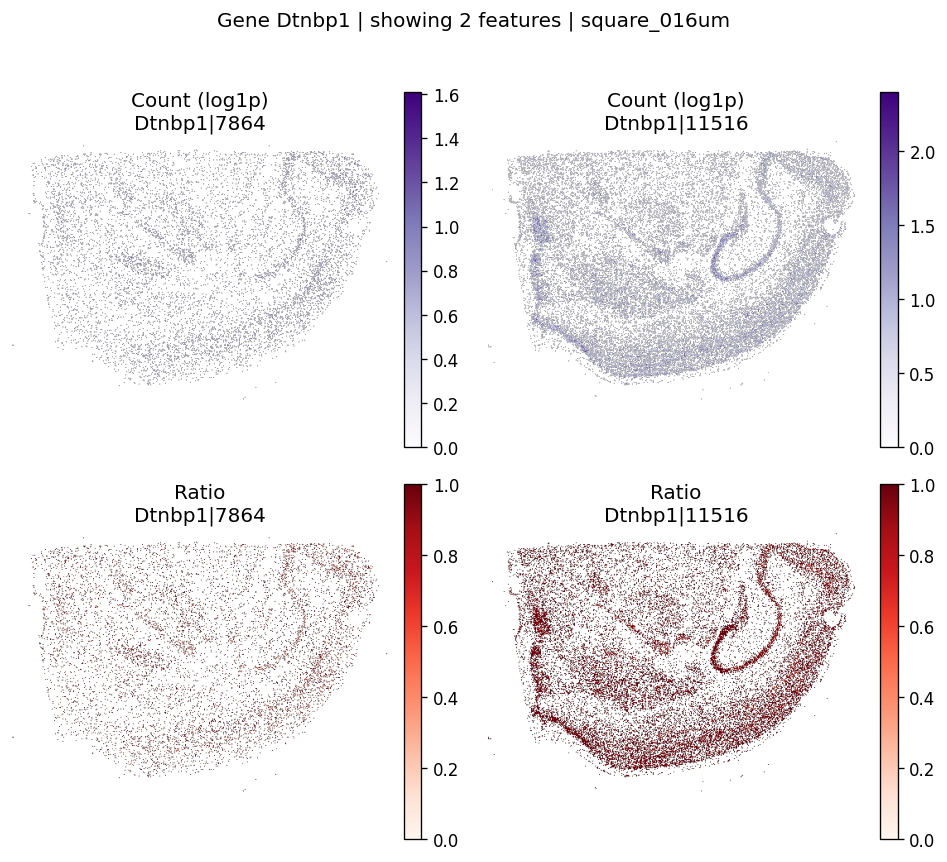
%%time
# Example: inspect a specific gene manually
plot_gene_codeword_maps(
    sdata=sdata,
    bin_table=test_table,
    bin_element=test_bins_element,
    gene_id='Dtnbp1',
    var_meta=sdata.tables[test_table].var,
    group_col=group_iso_by,
    max_features=6,
    hide_zero_ratio=True,
)

CPU times: user 239 ms, sys: 12.4 ms, total: 251 ms
Wall time: 251 ms

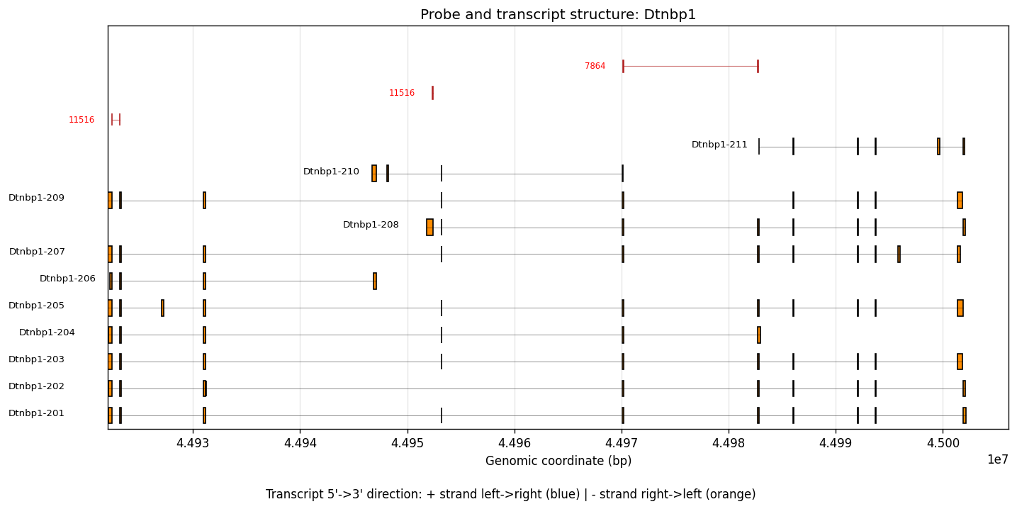
To see the spatially variable transcript regions, we can visualize the 10x reference probe sets along with a matched transcript reference. The following files need to be downloaded and provided as input:

• xenium_mouse_5K_gene_expression_panel_probe_locations.bed from 10x Genomics

• gencode.vM23.annotation.gtf.gz from GENCODE

Show code cell source

Hide code cell source

def plot_codeword_transcript_structure(
    gene_name: str,
    bed_file: str | Path,
    gtf_file: str | Path,
    figsize: tuple[float, float] = (12, 6),
):
    """Visualize codeword probes and transcript exon structure for one gene."""
    import gzip

    bed_file = Path(bed_file)
    gtf_file = Path(gtf_file)

    # Parse BED12/bedDetail rows while skipping track/browser headers.
    bed_cols = [
        "chrom",
        "start",
        "end",
        "name",
        "score",
        "strand",
        "thickStart",
        "thickEnd",
        "itemRgb",
        "blockCount",
        "blockSizes",
        "blockStarts",
        "detail",
    ]
    bed_records: list[list[str]] = []
    with open(bed_file, "rt", encoding="utf-8") as handle:
        for line in handle:
            line = line.rstrip("\n")
            if not line or line.startswith("#") or line.startswith("track") or line.startswith("browser"):
                continue
            parts = line.split("\t")
            if len(parts) < 12:
                continue
            detail = parts[12] if len(parts) >= 13 else ""
            bed_records.append(parts[:12] + [detail])

    if not bed_records:
        warnings.warn(f"No valid BED12 rows found in {bed_file}")
        return

    bed_df = pd.DataFrame(bed_records, columns=bed_cols)
    numeric_cols = ["start", "end", "thickStart", "thickEnd", "blockCount"]
    for col in numeric_cols:
        bed_df[col] = pd.to_numeric(bed_df[col], errors="coerce").fillna(0).astype(int)

    # Extract gene symbol, gene id, and codeword id from Xenium probe naming.
    def parse_probe_fields(row: pd.Series) -> pd.Series:
        name_text = str(row["name"])
        detail_text = str(row.get("detail", ""))

        parts = [p.strip() for p in name_text.split("|")]
        gene_token = parts[0] if parts else name_text
        codeword_id = parts[1] if len(parts) >= 2 else ""

        gene_symbol = gene_token.split(" (", 1)[0].strip()
        gene_id = ""
        if "(" in gene_token and ")" in gene_token:
            gene_id = gene_token.split("(", 1)[1].split(")", 1)[0].strip()

        if (not codeword_id) and ("Codeword:" in detail_text):
            codeword_id = detail_text.split("Codeword:", 1)[1].split(",", 1)[0].strip()

        if not codeword_id:
            codeword_id = "NA"

        return pd.Series(
            {
                "gene_symbol": gene_symbol,
                "gene_id": gene_id,
                "codeword_id": codeword_id,
            }
        )

    parsed = bed_df.apply(parse_probe_fields, axis=1)
    bed_df = pd.concat([bed_df, parsed], axis=1)

    # Match by gene symbol, Ensembl gene ID, or generic name contains fallback.
    gene_key = str(gene_name).strip().lower()
    probes = bed_df[
        (bed_df["gene_symbol"].str.lower() == gene_key)
        | (bed_df["gene_id"].str.lower() == gene_key)
        | (bed_df["name"].str.lower().str.contains(gene_key, na=False))
    ].copy()

    if probes.empty:
        warnings.warn(f"No probes found for gene '{gene_name}' in {bed_file}")

    # Convert BED12 blocks to absolute genomic coordinates per probe row.
    def parse_blocks(row: pd.Series) -> list[tuple[int, int]]:
        starts = [int(x) for x in str(row["blockStarts"]).strip(",").split(",") if x != ""]
        sizes = [int(x) for x in str(row["blockSizes"]).strip(",").split(",") if x != ""]
        n = min(int(row["blockCount"]), len(starts), len(sizes))

        if n == 0:
            return [(int(row["start"]), int(row["end"]))]

        blocks = []
        for i in range(n):
            block_start = int(row["start"]) + starts[i]
            block_end = block_start + sizes[i]
            blocks.append((block_start, block_end))
        return blocks

    if not probes.empty:
        probes["blocks"] = probes.apply(parse_blocks, axis=1)

    # Read GTF and filter transcripts by gene symbol or gene id.
    if str(gtf_file).endswith(".gz"):
        gtf_opener = lambda f: gzip.open(f, "rt")
    else:
        gtf_opener = open

    transcripts_by_id = {}
    with gtf_opener(gtf_file) as f:
        for line in f:
            if line.startswith("#"):
                continue
            fields = line.rstrip("\n").split("\t")
            if len(fields) < 9:
                continue
            ftype, start, end = fields[2], int(fields[3]), int(fields[4])
            attrs = {}
            for attr in fields[8].split("; "):
                if " " in attr:
                    k, v = attr.split(" ", 1)
                    attrs[k] = v.strip('"')

            if attrs.get("gene_name", "").lower() != gene_key and attrs.get("gene_id", "").lower() != gene_key:
                continue

            tx_id = attrs.get("transcript_id", "unknown")
            if tx_id not in transcripts_by_id:
                tx_name = attrs.get("transcript_name", tx_id)
                transcripts_by_id[tx_id] = {
                    "chrom": fields[0],
                    "strand": fields[6],
                    "tx_name": tx_name,
                    "exons": [],
                }

            if ftype == "exon":
                transcripts_by_id[tx_id]["exons"].append((start, end))

    fig, ax = plt.subplots(figsize=figsize)

    # Plot transcripts first.
    y_pos = 0
    x_mins: list[int] = []
    x_maxs: list[int] = []

    strand_colors = {
        "+": "steelblue",
        "-": "darkorange",
    }

    if transcripts_by_id:
        for tx_id, tx_info in sorted(transcripts_by_id.items()):
            exons = sorted(tx_info["exons"])
            if not exons:
                continue

            min_coord = min(e[0] for e in exons)
            max_coord = max(e[1] for e in exons)
            x_mins.append(min_coord)
            x_maxs.append(max_coord)
            ax.plot([min_coord, max_coord], [y_pos, y_pos], "k-", linewidth=0.5, alpha=0.5)

            strand = str(tx_info.get("strand", "."))
            tx_color = strand_colors.get(strand, "gray")
            for exon_start, exon_end in exons:
                ax.barh(y_pos, exon_end - exon_start, left=exon_start, height=0.6, color=tx_color, edgecolor="black")

            # Label with transcript_name
            tx_name = tx_info.get("tx_name", tx_id[:20])
            ax.text(min_coord - (max_coord - min_coord) * 0.05, y_pos, tx_name[:30], ha="right", fontsize=8)
            y_pos += 1

    # Keep one row per probe record, but use only codeword IDs as labels.
    probe_rows_for_plot: list[tuple[str, list[tuple[int, int]]]] = []
    if not probes.empty:
        probe_rows = probes.sort_values(["codeword_id", "chrom", "start", "end"])
        for _, row in probe_rows.iterrows():
            blocks = row["blocks"] if isinstance(row["blocks"], list) and row["blocks"] else [(int(row["start"]), int(row["end"]))]
            codeword_id = str(row.get("codeword_id", "NA"))
            probe_rows_for_plot.append((codeword_id, blocks))

            x_mins.append(min(s for s, _ in blocks))
            x_maxs.append(max(e for _, e in blocks))

    x_pad = max(1.0, (max(x_maxs) - min(x_mins)) * 0.02) if x_mins and x_maxs else 1.0

    for idx, (codeword_id, blocks) in enumerate(probe_rows_for_plot):
        probe_y = y_pos + idx
        probe_min = min(b[0] for b in blocks)
        probe_max = max(b[1] for b in blocks)

        ax.plot([probe_min, probe_max], [probe_y, probe_y], color="firebrick", linewidth=0.7, alpha=0.6)
        for block_start, block_end in blocks:
            ax.barh(
                probe_y,
                block_end - block_start,
                left=block_start,
                height=0.45,
                color="salmon",
                edgecolor="firebrick",
            )

        # Show codeword id only.
        ax.text(probe_min - x_pad, probe_y, codeword_id, ha="right", va="center", fontsize=7, color="red")

    y_pos += len(probe_rows_for_plot)

    ax.set_ylim(-0.5, y_pos + 0.5)
    ax.set_xlabel("Genomic coordinate (bp)")
    ax.set_ylabel("")
    ax.set_yticks([])
    ax.set_title(f"Probe and transcript structure: {gene_name}")
    ax.grid(True, axis="x", alpha=0.3)

    direction_note = "Transcript 5'->3' direction: + strand left->right (blue) | - strand right->left (orange)"
    fig.text(0.5, 0.01, direction_note, ha="center", va="bottom", fontsize=10, color="black")

    fig.tight_layout(rect=(0.0, 0.05, 1.0, 1.0))
    plt.show()

%%time
plot_codeword_transcript_structure(
    gene_name="Dtnbp1",
    bed_file=bed_file,
    gtf_file=gtf_file,
)

CPU times: user 6.27 s, sys: 59.9 ms, total: 6.33 s
Wall time: 6.39 s

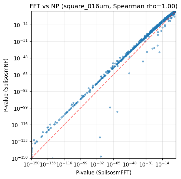
Method comparison: SplisosmFFT vs SplisosmNP

We now compare FFT-accelerated and non-parametric spatial variability tests on the same AnnData table.

Note: Since v1.2.0, SplisosmNP SV tests use Liu’s approximation from full-rank spatial-kernel cumulants by default. See the SV hyperparameter optimization notebook for comparison with the legacy low-rank approach.

For large implicit CAR kernels, null_configs={"n_probes": m} controls the Hutchinson trace budget. Smaller m is faster but noisier. To emphasize broad smooth patterns, prefer increasing rho (for example, rho=0.999) rather than rank truncation.

%%time
model_np = SplisosmNP(
    k_neighbors=4,
    rho=0.99,
    standardize_cov=False # turn off for faster runtime
)
model_np.setup_data(
    adata=sdata.tables[test_table],
    spatial_key='spatial',
    layer='counts',
    group_iso_by=group_iso_by,
    gene_names=gene_name_col,
    min_counts=min_counts,
    min_bin_pct=min_bin_pct,
    min_component_size=10 # remove disconnected tissue fragments if any
)
model_np

CPU times: user 1.41 s, sys: 405 ms, total: 1.81 s
Wall time: 1.88 s

=== SplisosmNP
- Number of genes: 4972
- Number of spots: 144372
- Number of covariates: 0
- Average isoforms per gene: 2.1
=== Model configurations
- Spatial kernel source: spatial_key='spatial' (component-filtered)
- k_neighbors: 4, rho: 0.99
- Standardize spatial covariance: False
=== Test results
- Spatial variability: N/A
- Differential usage: N/A

%%time
model_np.test_spatial_variability(
    method='hsic-ir',
    null_configs={"n_probes": 60},
    ratio_transformation='none',
    print_progress=True,
)

SV [hsic-ir]: 100%|██████████| 331/331 [00:14<00:00, 22.85it/s]

CPU times: user 1min 41s, sys: 10.6 s, total: 1min 52s
Wall time: 16.2 s

sv_np = model_np.get_formatted_test_results('sv')[['gene', 'pvalue']].copy()
sv_np = sv_np.rename(columns={'pvalue': 'pvalue_np'})

comparison = sv_res_fft[['gene', 'pvalue']].copy()
comparison = comparison.rename(columns={'pvalue': 'pvalue_fft'})
comparison = comparison.merge(sv_np, on='gene', how='inner')

corr, _ = spearmanr(comparison['pvalue_fft'], comparison['pvalue_np'])

print(f'Genes tested in both methods: {len(comparison)}')
print(f'P-value correlation (Spearman rho): {corr:.4f}')

Genes tested in both methods: 4972
P-value correlation (Spearman rho): 0.9985

fig, ax = plt.subplots(figsize=(5, 5))
x = comparison['pvalue_fft'].to_numpy()
y = comparison['pvalue_np'].to_numpy()

ax.scatter(x + 1e-150, y + 1e-150, s=8, alpha=0.5)
ax.set_xscale('log')
ax.set_yscale('log')
ax.set_xlabel('P-value (SplisosmFFT)')
ax.set_ylabel('P-value (SplisosmNP)')
ax.set_title(f'FFT vs NP ({test_table}, Spearman rho={corr:.2f})')
ax.grid(True, alpha=0.3)

lims = [1e-150, 1.0]
ax.plot(lims, lims, 'r--', alpha=0.5, linewidth=1.5)
ax.set_xlim(lims)
ax.set_ylim(lims)

plt.tight_layout()
plt.show()

Summary

• load_xenium_codeword enables direct codeword-level multi-resolution binning from Xenium outputs.

• SplisosmFFT is an efficient default on regular square grids and yield highly similar results to SplisosmNP.

For reproducibility

import sys
from datetime import date
import splisosm

print('Last updated:', date.today())
print('Python:', sys.version.split()[0])
print('splisosm:', getattr(splisosm, '__version__', 'unknown'))

Last updated: 2026-05-03
Python: 3.12.13
splisosm: 1.2.0rc1