Visium HD FFPE (probe) Part II

This notebook is the second of two tutorials where we apply SPLISOSM to a probe-based Visium HD FFPE dataset of adult mouse brain. It covers the following steps:

1. Run spatial variability (SV) tests to find genes with spatially variable probe usage, and RBP genes with spatially variable expression.

2. For spatially variably processed (SVP) genes, run differential usage (DU) tests to check whether the probe usage co-varies with SV-RBP expression.

3. Compare results of conditional and non-conditional differential usage tests, and between SplisosmFFT (rasterized) and SplisosmNP (vectorized) implementations.

Previous step: Visium HD FFPE (probe) Part I for data loading and SV test details.

The workflow is compatible with other ST platforms. See guidance on data preparation and the tutorial gallery for more examples.

Estimated runtime: ~10 min.

Preliminary notes

The differential association tests here ask whether RBP expression and probe usage are associated within the same bin. They do not test cross-bin association, such as whether an RBP in one subcellular bin is associated with probe usage in neighboring bins. For that reason, use 16 µm bins or coarser for this analysis.

Imports

from __future__ import annotations

from pathlib import Path
import warnings

import numpy as np
import pandas as pd
import matplotlib.pyplot as plt
from scipy.stats import spearmanr
import scipy.sparse as sp

import spatialdata as sd
from spatialdata import rasterize_bins
from spatialdata.models import TableModel
from anndata import AnnData

from splisosm import SplisosmFFT, SplisosmNP
from splisosm.io import load_visiumhd_probe
from splisosm.utils import counts_to_ratios

warnings.filterwarnings("ignore", category=FutureWarning)
plt.rcParams["figure.dpi"] = 120
plt.rcParams["figure.figsize"] = (6, 4)

Configure paths and parameters

Here, we focus on a list of potential RNA processing regulators, which are RBP genes with either CLIP data from POSTAR3 or binding motifs from CISBP-RNA. Feel free to modify the RBP gene list and create your own covariate table as needed.

# # RBP reference files
# rbp_motif_file = Path("path/to/cisbp-rna/mouse_pm/rbp_with_known_motif.txt")
# rbp_clip_file  = Path("path/to/POSTAR3/mouse.rbp_with_clip.txt")
# rbp_motif_genes = set(pd.read_csv(rbp_motif_file, header=None).iloc[:, 0].str.strip())
# rbp_clip_genes  = set(pd.read_csv(rbp_clip_file,  header=None).iloc[:, 0].str.strip())
# rbp_genes       = rbp_motif_genes | rbp_clip_genes
# print(f"CisBP-RNA (motif): {len(rbp_motif_genes)}  |  POSTAR3 (CLIP): {len(rbp_clip_genes)}")

rbp_genes = {
    'A1cf', 'Ago2', 'Ankhd1', 'Ankrd17', 'Apc', 'B020018G12Rik', 'Cbp', 'Celf',
    'Celf1', 'Celf2', 'Celf3', 'Celf4', 'Celf6', 'Cirbp', 'Cnot4', 'Cpeb2',
    'Cpeb3', 'Cpeb4', 'Cpsf6', 'Crebbp', 'Csda', 'Dazap1', 'ENSMUSG00000021927',
    'ENSMUSG00000049235', 'ENSMUSG00000056951', 'ENSMUSG00000089986',
    'ENSMUSG00000090049', 'Eif2s1', 'Eif4b', 'Elavl1', 'Elavl2', 'Elavl3',
    'Elavl4', 'Enox1', 'Enox2', 'Esrp1', 'Esrp2', 'Ezh2', 'Fam120a', 'Fmr1',
    'Fus', 'Fxr1', 'Fxr2', 'G3bp2', 'Gm10110', 'Gm12355', 'Gm5145', 'Gm7964',
    'Gm8991', 'Hnrnpa1', 'Hnrnpa2b1', 'Hnrnpa3', 'Hnrnpab', 'Hnrnpc', 'Hnrnpf',
    'Hnrnph1', 'Hnrnph2', 'Hnrnpk', 'Hnrnpl', 'Hnrnpr', 'Hnrpdl', 'Hnrpll',
    'Igf2bp1', 'Igf2bp2', 'Igf2bp3', 'Khdrbs1', 'Khdrbs2', 'Khdrbs3', 'Lin28a',
    'Lin28b', 'Matr3', 'Mbnl1', 'Mbnl2', 'Mbnl3', 'Mex3b', 'Mex3c', 'Mex3d',
    'Msi1', 'Msi2', 'Ncl', 'Nono', 'Nova1', 'Nova2', 'Pabpc1', 'Pabpc1l',
    'Pabpc2', 'Pabpc4', 'Pabpc5', 'Pabpc6', 'Pabpn1', 'Pcbp1', 'Pcbp2', 'Pcbp3',
    'Pcbp4', 'Pou5f1', 'Pprc1', 'Pspc1', 'Ptbp1', 'Ptbp2', 'Pum1', 'Pum2', 'Qk',
    'Raly', 'Ralyl', 'Rbfox1', 'Rbfox2', 'Rbfox3', 'Rbm10', 'Rbm24', 'Rbm28',
    'Rbm3', 'Rbm38', 'Rbm41', 'Rbm42', 'Rbm45', 'Rbm46', 'Rbm47', 'Rbm4b',
    'Rbm5', 'Rbm8a', 'Rbms1', 'Rbms2', 'Rbms3', 'Rbmx', 'Rbmxl2', 'Rbmxrt',
    'Rod1', 'Samd4', 'Samd4b', 'Sart3', 'Sf3b4', 'Sfpq', 'Snrnp70', 'Snrpa',
    'Snrpb2', 'Srrm4', 'Srsf1', 'Srsf10', 'Srsf12', 'Srsf2', 'Srsf3', 'Srsf4',
    'Srsf5', 'Srsf6', 'Srsf7', 'Srsf9', 'Syncrip', 'Taf15', 'Tardbp', 'Tia1',
    'Tial1', 'Ttp', 'Tut1', 'U2af2', 'Upf1', 'Ybx1', 'Ybx2', 'Ythdc1', 'Ythdc2',
    'Yy1', 'Zc3h10', 'Zcrb1', 'Zfp36', 'Zfp36l1', 'Zfp36l2', 'Zfp36l3'
}

print(f"Union: {len(rbp_genes)} RBP genes")

Union: 166 RBP genes

# Required: Space Ranger `outs` directory for Visium HD
visium_hd_outs = Path("/path/to/visium_hd_ffpe/outs")
sdata_zarr     = visium_hd_outs / "sdata_probe.filtered.zarr"

# Dataset / table identifiers — 16 µm throughout
dataset_id        = "Visium_HD_Mouse_Brain"
test_table        = "square_016um"
test_bins_element = f"{dataset_id}_square_016um"

# Probe annotation columns
group_iso_by           = "gene_ids"
candidate_gene_name_cols = ["gene_name", "gene_symbol", "gene_names"]

# Probe QC filters
min_counts  = 10
min_bin_pct = 0.01

Load SpatialData

%%time
# Load preprocessed SpatialData object with probe-level quantification
sdata = sd.read_zarr(sdata_zarr)

# Check the presence of the test table and the required columns
adata_probe = sdata.tables[test_table]
if group_iso_by not in adata_probe.var.columns:
    raise ValueError(f"{group_iso_by!r} not found in {test_table}.var")

gene_name_col = next(
    (c for c in candidate_gene_name_cols if c in adata_probe.var.columns), None
)
if gene_name_col is None:
    raise ValueError(f"None of {candidate_gene_name_cols} found in adata_probe.var")

print(f"table={test_table}  bins={test_bins_element}")
print(f"group_iso_by={group_iso_by!r}  gene_name_col={gene_name_col!r}")
print(f"Probes: {adata_probe.n_vars}   Spots: {adata_probe.n_obs}")

table=square_016um  bins=Visium_HD_Mouse_Brain_square_016um
group_iso_by='gene_ids'  gene_name_col='gene_name'
Probes: 55538   Spots: 98917
CPU times: user 8.1 s, sys: 1.46 s, total: 9.55 s
Wall time: 5.53 s

Spatial variability tests

Find genes with spatially variable probe usage (same as Part I)

We first test each multi-probe gene for spatially variable probe usage (within-gene ratios) using SplisosmFFT and method="hsic-ir"at 16 µm resolution.

%%time
model_sv = SplisosmFFT(neighbor_degree=1, rho=0.99)
model_sv.setup_data(
    sdata=sdata,
    bins=test_bins_element,
    table_name=test_table,
    col_key="array_col",
    row_key="array_row",
    layer="counts",
    group_iso_by=group_iso_by,
    gene_names=gene_name_col,
    min_counts=min_counts,
    min_bin_pct=min_bin_pct,
    filter_single_iso_genes=True,
)
model_sv.test_spatial_variability(
    method="hsic-ir",
    ratio_transformation="none",
    n_jobs=-1,
    print_progress=True,
)

SV [hsic-ir]: 100%|██████████| 551/551 [00:25<00:00, 21.77it/s]

CPU times: user 1min 30s, sys: 18.8 s, total: 1min 48s
Wall time: 31 s

# Define SV genes for DU targets based on FFT results (FDR < 0.01)
sv_res_fft = model_sv.get_formatted_test_results(
      "sv", with_gene_summary=True
).sort_values("pvalue_adj")
sv_probe_gene_list = sorted(set(sv_res_fft.loc[sv_res_fft["pvalue_adj"] < 0.01, "gene"].astype(str)))
print(f"SVP genes (FFT FDR<0.01): {len(sv_probe_gene_list)} / {len(sv_res_fft)} \n"
      f"Will use these {len(sv_probe_gene_list)} genes as downstream DU targets")

sv_res_fft.head(5)

SVP genes (FFT FDR<0.01): 196 / 6226 
Will use these 196 genes as downstream DU targets

	gene	statistic	pvalue	pvalue_adj	n_isos	perplexity	pct_bin_on	count_avg	count_std	major_ratio_avg
3964	Syt1	0.000003	0.000000e+00	0.000000e+00	3	2.628424	0.387153	0.758151	1.310308	0.584887
3517	Map4	0.000005	0.000000e+00	0.000000e+00	6	5.579242	0.347968	0.494172	0.839410	0.268749
1805	Gabbr1	0.000003	1.127522e-258	2.339232e-255	6	5.344769	0.283450	0.401003	0.768475	0.262467
1463	Oxr1	0.000002	1.331162e-135	2.071288e-132	5	4.394658	0.203888	0.274887	0.630308	0.306204
2276	Rabgap1l	0.000003	1.409530e-81	1.754583e-78	6	5.325925	0.242779	0.335079	0.701223	0.279439

Find RBP genes with spatially variable expression

We next test each RBP gene for spatially variable expression using SplisosmFFT and method="hsic-gc" at 16 µm resolution. Spatially variably expressed RBP genes will be used as covariates in the downstream conditional DU test.

First, build gene-level RBP table (sum probe counts to gene-level) and save to the same SpatialData object.

%%time
# Filter probes to RBP genes
probe_gene_arr = adata_probe.var[gene_name_col].values
present_rbp = sorted(g for g in rbp_genes if g in set(probe_gene_arr))
print(f"RBP genes in dataset: {len(present_rbp)} / {len(rbp_genes)}")

# Define probe → gene mapping for present RBP genes
rbp_probe_mask = adata_probe.var[gene_name_col].isin(present_rbp).values
probe_gene_sub = adata_probe.var.loc[rbp_probe_mask, gene_name_col].values
unique_rbp_genes = sorted(set(probe_gene_sub))
gene_to_idx = {g: i for i, g in enumerate(unique_rbp_genes)}
probe_to_gene = np.array([gene_to_idx[g] for g in probe_gene_sub])

n_rbp_probe = int(rbp_probe_mask.sum())
agg_mat = sp.csr_matrix(
    (np.ones(n_rbp_probe), (probe_to_gene, np.arange(n_rbp_probe))),
    shape=(len(unique_rbp_genes), n_rbp_probe),
)

# Sum probe counts → gene counts: (n_spots, n_rbp)
X_rbp_probes = adata_probe.layers["counts"].tocsr()[:, rbp_probe_mask]
X_rbp_genes = (X_rbp_probes @ agg_mat.T).tocsc()   # csc for rasterize_bins

# Build obs (copy spatial metadata from probe table)
var_df_rbp = pd.DataFrame({
    "gene_name": unique_rbp_genes,
    "gene_ids": unique_rbp_genes,  # dummy gene_ids
}, index=unique_rbp_genes)

adata_rbp = AnnData(
    X=X_rbp_genes,
    obs=adata_probe.obs.copy(),
    var=var_df_rbp,
    # copy over spatialdata_attrs for parsing region/instance keys
    uns=adata_probe.uns.copy(),
    obsm=adata_probe.obsm.copy(),
)
adata_rbp.layers["counts"] = X_rbp_genes
print(f"RBP gene table: {adata_rbp.n_obs} spots × {adata_rbp.n_vars} genes")

RBP genes in dataset: 143 / 166
RBP gene table: 98917 spots × 143 genes
CPU times: user 198 ms, sys: 5.64 ms, total: 203 ms
Wall time: 206 ms

# Add gene-level RBP table to SpatialData
sdata["square_016um_rbp_genes"] = TableModel.parse(adata_rbp)
sdata

SpatialData object, with associated Zarr store: /Users/jysumac/Projects/SPLISOSM_paper/data/visiumhd_ffpe_mouse_cbs/sdata_probe.filtered.zarr
├── Images
│     ├── 'Visium_HD_Mouse_Brain_full_image': DataTree[cyx] (3, 23947, 18872), (3, 11973, 9436), (3, 5986, 4718), (3, 2993, 2359), (3, 1496, 1179)
│     ├── 'Visium_HD_Mouse_Brain_hires_image': DataArray[cyx] (3, 6000, 4729)
│     ├── 'Visium_HD_Mouse_Brain_lowres_image': DataArray[cyx] (3, 600, 473)
│     └── 'rasterized_square_016um_counts': DataArray[cyx] (55538, 396, 314)
├── Shapes
│     ├── 'Visium_HD_Mouse_Brain_cell_segmentations': GeoDataFrame shape: (40222, 2) (2D shapes)
│     ├── 'Visium_HD_Mouse_Brain_square_002um': GeoDataFrame shape: (6296688, 1) (2D shapes)
│     ├── 'Visium_HD_Mouse_Brain_square_008um': GeoDataFrame shape: (393543, 1) (2D shapes)
│     └── 'Visium_HD_Mouse_Brain_square_016um': GeoDataFrame shape: (98917, 1) (2D shapes)
└── Tables
      ├── 'cell_segmentations': AnnData (40222, 55538)
      ├── 'square_002um': AnnData (6296688, 55538)
      ├── 'square_008um': AnnData (393543, 55538)
      ├── 'square_016um': AnnData (98917, 55538)
      └── 'square_016um_rbp_genes': AnnData (98917, 143)
with coordinate systems:
    ▸ 'Visium_HD_Mouse_Brain', with elements:
        Visium_HD_Mouse_Brain_full_image (Images), Visium_HD_Mouse_Brain_hires_image (Images), Visium_HD_Mouse_Brain_lowres_image (Images), rasterized_square_016um_counts (Images), Visium_HD_Mouse_Brain_cell_segmentations (Shapes), Visium_HD_Mouse_Brain_square_002um (Shapes), Visium_HD_Mouse_Brain_square_008um (Shapes), Visium_HD_Mouse_Brain_square_016um (Shapes)
    ▸ 'Visium_HD_Mouse_Brain_downscaled_hires', with elements:
        Visium_HD_Mouse_Brain_hires_image (Images), rasterized_square_016um_counts (Images), Visium_HD_Mouse_Brain_cell_segmentations (Shapes), Visium_HD_Mouse_Brain_square_002um (Shapes), Visium_HD_Mouse_Brain_square_008um (Shapes), Visium_HD_Mouse_Brain_square_016um (Shapes)
    ▸ 'Visium_HD_Mouse_Brain_downscaled_lowres', with elements:
        Visium_HD_Mouse_Brain_lowres_image (Images), rasterized_square_016um_counts (Images), Visium_HD_Mouse_Brain_cell_segmentations (Shapes), Visium_HD_Mouse_Brain_square_002um (Shapes), Visium_HD_Mouse_Brain_square_008um (Shapes), Visium_HD_Mouse_Brain_square_016um (Shapes)
with the following elements not in the Zarr store:
    ▸ rasterized_square_016um_counts (Images)
    ▸ square_016um_rbp_genes (Tables)

Next, we run the SVE test (method="hsic-gc") for RBP gene expression. Here, filter_single_iso_genes=False keeps genes with only one feature, which is the case for all RBP genes since we have aggregated probe counts to the total count.

%%time
rbp_sv = SplisosmFFT()
rbp_sv.setup_data(
    sdata=sdata,
    bins=test_bins_element,
    table_name="square_016um_rbp_genes",
    col_key="array_col",
    row_key="array_row",
    layer="counts",
    group_iso_by=gene_name_col,
    gene_names=gene_name_col,
    min_counts=min_counts,
    min_bin_pct=min_bin_pct,
    filter_single_iso_genes=False,  # every gene has exactly one entry (no probe-level info)
)
rbp_sv.test_spatial_variability(
    method="hsic-gc",
    print_progress=True,
)

SV [hsic-gc]: 100%|██████████| 4/4 [00:00<00:00, 46474.28it/s]

CPU times: user 696 ms, sys: 102 ms, total: 798 ms
Wall time: 327 ms

%%time
sv_res_rbp = rbp_sv.get_formatted_test_results("sv").sort_values("pvalue_adj")
sv_rbp_names = sv_res_rbp.loc[sv_res_rbp["pvalue_adj"] < 0.01, "gene"].astype(str).tolist()
print(f"Spatially variable RBP genes (FDR < 0.01): {len(sv_rbp_names)} / {len(sv_res_rbp)}")
sv_res_rbp.tail(5)

Spatially variable RBP genes (FDR < 0.01): 125 / 125
CPU times: user 570 μs, sys: 43 μs, total: 613 μs
Wall time: 621 μs

	gene	statistic	pvalue	pvalue_adj
120	Zc3h10	3.426719e-07	7.296523e-122	7.537730e-122
86	Rbms2	4.263304e-07	1.076983e-112	1.103466e-112
82	Rbm4b	2.577039e-07	4.921084e-109	5.001102e-109
79	Rbm41	2.310365e-07	4.441879e-83	4.477700e-83
24	Ezh2	2.376248e-07	1.453297e-48	1.453297e-48

Differential probe usage vs RBP expression

In this section, we will test whether the usage of different probes for each spatially variably processed (SVP, FDR < 0.01) gene is associated with the expression of spatially variable RBP genes. A significant result may indicate the potential regulator of variable probe usage events. However, spatial autocorrelation is a major confounder that can lead to spurious associations. For example, RBP expression may correlate with some probe usage due to underlying hidden spatial structure such as cell-type distribution. To address this, we will compare two approaches:

• Non-conditional test (method="hsic"): tests raw probe ratios vs raw RBP expression through the multivariate correlation coefficient.

• Conditional test (method="hsic-gp"): tests usage association after removing confounding spatial structure using FFT-accelerated Gaussian process regression.

Prepare filtered probe table (SVP genes only)

# Restrict probe table to SV-processed genes for the DU test
sv_probe_mask_var = adata_probe.var[gene_name_col].isin(sv_probe_gene_list)
adata_probe_svp = adata_probe[:, sv_probe_mask_var].copy()
print(f"Filtered probe table: {adata_probe_svp.n_obs} spots x {adata_probe_svp.n_vars} probes "
      f"({len(sv_probe_gene_list)} genes)")

sdata["square_016um_svp"] = TableModel.parse(adata_probe_svp)

Filtered probe table: 98917 spots x 661 probes (196 genes)

Register the covariate table

To run the differential usage test, you must pass a (n_spots, n_covariates) design matrix to SplisosmFFT.setup_data(). This can be provided in one of three ways:

1. An AnnData table from the SpatialData object (e.g., the sdata.tables['square_016um_rbp_genes'] table we just registered). All features in table.var will be used as covariates.

2. A list of column names from in the AnnData’s .obs (e.g., adata_probe_svp.obs.columns). Categorical columns will be automatically one-hot encoded.

3. A user-provided DataFrame/array-like design matrix that shares the same spot indices as the data (e.g., adata_probe_svp.obs_names).

To register a custom covariate design matrix directly within your SpatialData object, follow these steps:

1. Create an AnnData object with the covariate matrix in .X and spot IDs in .obs_names.

2. Add the required metadata (.uns['spatialdata_attrs'], .obsm) and mapping columns to .obs to align the table with your spatial elements.

3. Parse the AnnData object using TableModel.parse() (specifying region, region_key and instance_key) and add it to the SpatialData object. See the SpatialData documentation for further details.

# Since all RBP genes are spatially variably expressed, the following will
# duplicate the RBP covariate matrix as a new table in the SpatialData
adata_rbp_cov = adata_rbp[:, sv_rbp_names].copy()
adata_rbp_cov.X = adata_rbp_cov.layers["counts"].tocsc()

# adata_rbp_cov.uns["spatialdata_attrs"] is already copied from adata_rbp, 
# so the following will work without additional metadata adjustments
sdata["square_016um_rbp_sve"] = TableModel.parse(adata_rbp_cov)

Run conditional differential usage test

%%time
model_du_fft = SplisosmFFT(neighbor_degree=1, rho=0.99)
model_du_fft.setup_data(
    sdata=sdata,
    bins=test_bins_element, # the 16 µm bin for rasterization
    table_name="square_016um_svp", # probe counts from SVP genes
    design_mtx="square_016um_rbp_sve",    # gene counts from SVE RBPs
    col_key="array_col",
    row_key="array_row",
    layer="counts",
    group_iso_by=group_iso_by,
    gene_names=gene_name_col,
    min_counts=min_counts,
    min_bin_pct=min_bin_pct,
    filter_single_iso_genes=True, # same as the SVP test
)
print(model_du_fft)

=== SplisosmFFT
- Number of genes: 196
- Number of spots: 98917
- Number of spots after rasterization: 124344
- Number of covariates: 125
- Average isoforms per gene: 3.1
=== Model configurations
- Neighborhood degree: 1
- Spatial autocorrelation rho: 0.99
=== Test results
- Spatial variability: N/A
- Differential usage: N/A
CPU times: user 112 ms, sys: 8.27 ms, total: 120 ms
Wall time: 120 ms

%%time
# conditional DU test
model_du_fft.test_differential_usage(
    method='hsic-gp',
    residualize="cov_only",
    n_jobs=-1,
    print_progress=True,
)
du_fft = model_du_fft.get_formatted_test_results("du").sort_values("pvalue_adj")
n_sig_fft = int((du_fft["pvalue_adj"] < 0.01).sum())
print(f"Significant gene-RBP pairs (FDR < 0.01, multi-testing correction per RBP): {n_sig_fft} / {len(du_fft)}")
du_fft.head(10)

Covariates: 100%|██████████| 2/2 [00:08<00:00,  4.40s/it]

Significant gene-RBP pairs (FDR < 0.01, multi-testing correction per RBP): 2148 / 24500
CPU times: user 10.8 s, sys: 1.71 s, total: 12.6 s
Wall time: 8.83 s

	gene	covariate	statistic	pvalue	pvalue_adj
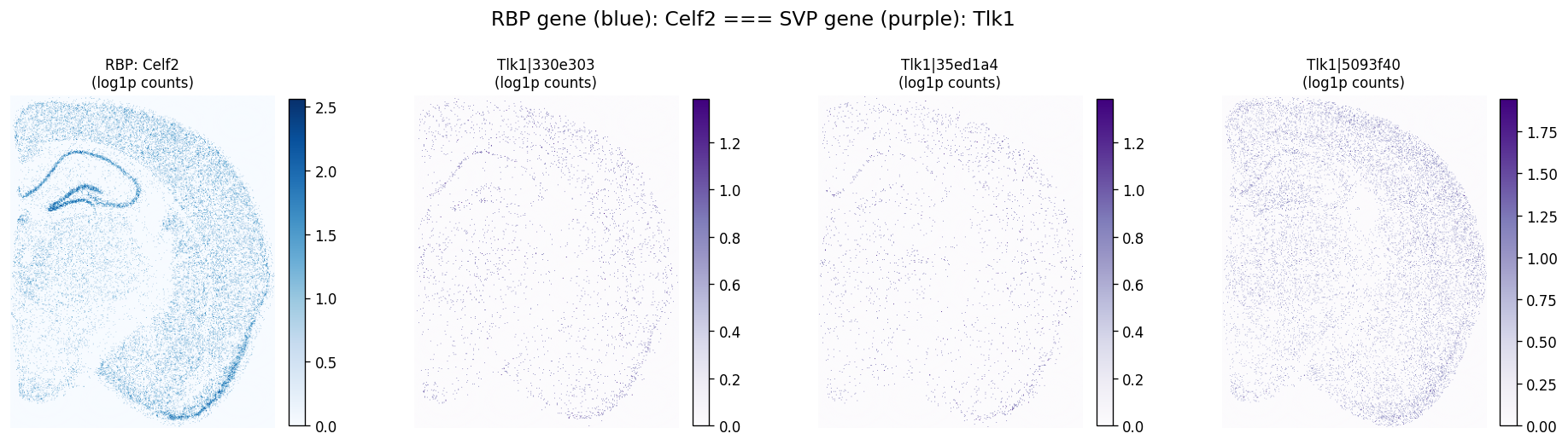
18827	Tlk1	Celf2	0.000051	1.329160e-41	2.605153e-39
14265	Map4	Ptbp2	0.000061	1.416121e-34	2.775598e-32
18799	Tlk1	Snrnp70	0.000038	2.361746e-31	4.629022e-29
18817	Tlk1	Dazap1	0.000035	3.226290e-29	6.323529e-27
14261	Map4	Ralyl	0.000050	1.717097e-28	3.365511e-26
14259	Map4	Rbfox2	0.000049	6.617653e-28	1.297060e-25
14314	Map4	Elavl2	0.000048	2.711018e-27	5.313596e-25
18760	Tlk1	Rbfox1	0.000033	4.701848e-27	9.215623e-25
18794	Tlk1	Srsf3	0.000032	9.226192e-27	1.808334e-24
14312	Map4	Elavl4	0.000047	1.866261e-26	3.657872e-24

Visualize top RBP-gene pairs

def ensure_rasterized(sdata, bin_table: str, bin_element: str, layer: str = "counts"):
    raster_key = f"rasterized_{bin_table}_{layer}"
    if raster_key in sdata.images:
        return raster_key

    adata = sdata.tables[bin_table]
    adata.X = adata.layers[layer]
    if hasattr(adata.X, "tocsc") and getattr(adata.X, "format", None) != "csc":
        adata.X = adata.X.tocsc()

    sdata[raster_key] = rasterize_bins(
        sdata,
        bins=bin_element,
        table_name=bin_table,
        col_key="array_col",
        row_key="array_row",
    )
    return raster_key

First take a look at the spatial expression of the top RBP-gene pair (Celf2-Tlk1) to see if their spatial patterns are visually correlated.

def plot_rbp_svp_pair(
    sdata,
    bin_element: str,
    rbp_table: str,
    rbp_gene: str,
    svp_table: str,
    svp_gene: str,
    svp_gene_col: str = "gene_ids",
    max_probes: int = 4,
): 
    """Plot RBP spatial expression alongside SVP gene probe count maps in one row.""" 
    # ── load RBP expression raster ────────────────────────────────────────── 
    rbp_raster_key = ensure_rasterized(sdata, rbp_table, bin_element)
    rbp_cube = np.asarray(
        sdata[rbp_raster_key].sel(c=[rbp_gene]).values[0], dtype=float
    ) # (ny, nx)
    
    # ── load SVP probe count raster ─────────────────────────────────────────
    adata_svp = sdata.tables[svp_table]
    probe_var = adata_svp.var.copy()
    probe_names = probe_var.index[
        probe_var[svp_gene_col].astype(str) == str(svp_gene)
    ].tolist()
    probe_names = [p for p in probe_names if p in adata_svp.var_names][:max_probes]
    
    if not probe_names: 
        raise ValueError(f"No probes found for '{svp_gene}' in column '{svp_gene_col}'")
        
    svp_raster_key = ensure_rasterized(sdata, svp_table, bin_element)
    probe_cube = np.moveaxis(
        np.asarray(sdata[svp_raster_key].sel(c=probe_names).values, dtype=float), 0, -1
    ) # (ny, nx, n_probes)
    
    n_probes = probe_cube.shape[-1]
    n_cols = 1 + n_probes
    fig, axes = plt.subplots(1, n_cols, figsize=(4 * n_cols, 4.2), squeeze=False) 
    
    # Panel 0: RBP expression 
    rbp_map = np.log1p(rbp_cube)
    im0 = axes[0, 0].imshow(rbp_map, cmap="Blues")
    axes[0, 0].set_title(f"RBP: {rbp_gene}\n(log1p counts)", fontsize=10)
    axes[0, 0].axis("off")
    fig.colorbar(im0, ax=axes[0, 0], fraction=0.046, pad=0.04)
    
    # Panels 1…n_probes: SVP probe counts
    for i, probe in enumerate(probe_names): 
        c = probe_cube[:, :, i]
        c_map = np.log1p(c) 
        im = axes[0, i + 1].imshow(c_map, cmap="Purples") 
        axes[0, i + 1].set_title(f"{probe}\n(log1p counts)", fontsize=10) 
        axes[0, i + 1].axis("off") 
        fig.colorbar(im, ax=axes[0, i + 1], fraction=0.046, pad=0.04) 
        
    fig.suptitle(f"RBP gene (blue): {rbp_gene} === SVP gene (purple): {svp_gene}", fontsize=14, y=1.01) 
    fig.tight_layout() 
    plt.show()

plot_rbp_svp_pair(
    sdata=sdata,
    bin_element=test_bins_element,
    rbp_table='square_016um_rbp_sve',
    rbp_gene='Celf2',
    svp_table='square_016um_svp',
    svp_gene='Tlk1',
    svp_gene_col=gene_name_col,
    max_probes=4,
)

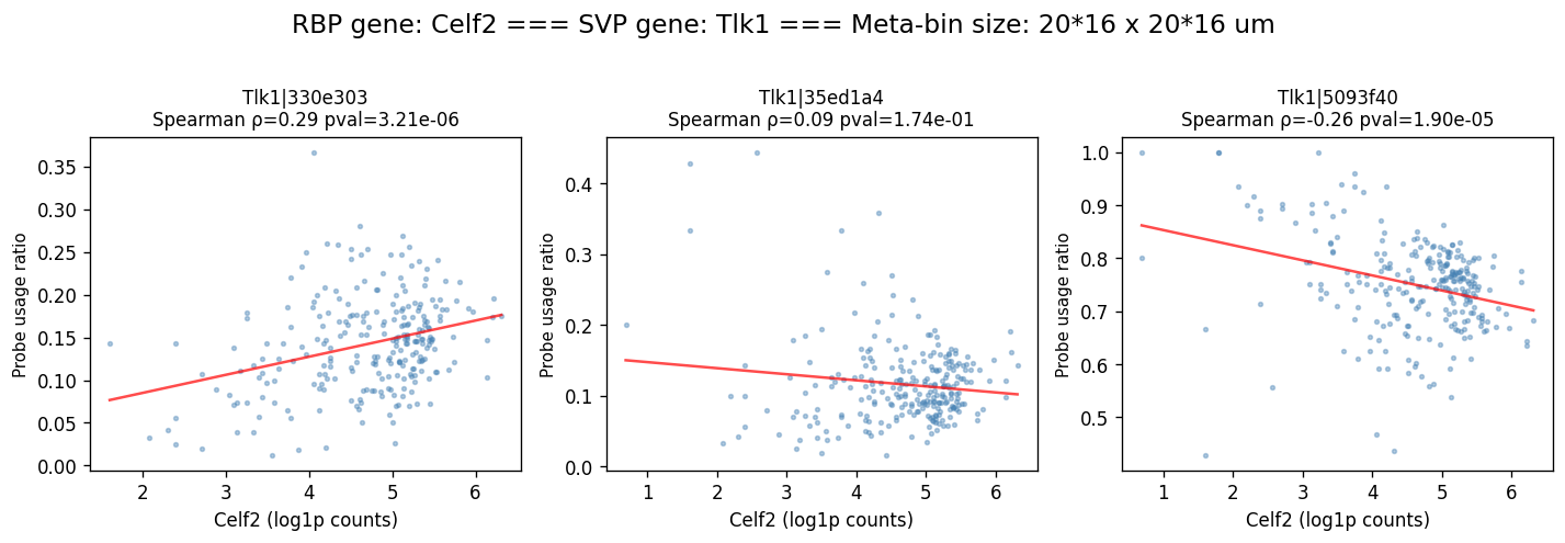
We can also plot probe usage ratios as a function of RBP expression. Since the raw 16 µm-bin data is very sparse and the counts and ratios are almost binary, we will aggregate adjacent bins into meta bins (meta_bin_size=4 gives 4 × 16 = 64 µm by 64 µm meta bins) to get more robust estimates of probe usage ratios and RBP expression.

def plot_rbp_vs_probe_scatter(
    sdata,
    bin_element: str,
    rbp_table: str,
    rbp_gene: str,
    svp_table: str,
    svp_gene: str,
    svp_gene_col: str = "gene_ids",
    max_probes: int = 4,
    meta_bin_size: int = 4,
): 
    """Scatter plot: RBP expression (x) vs per-probe usage ratio (y) using meta bins.""" 
    import torch as _torch 
    import numpy as np
    from scipy.stats import spearmanr
    import matplotlib.pyplot as plt
    
    # ── load RBP expression ──────────────────────────────────────────────────
    rbp_raster_key = ensure_rasterized(sdata, rbp_table, bin_element) 
    rbp_cube = np.asarray(
        sdata[rbp_raster_key].sel(c=[rbp_gene]).values[0], 
        dtype=float
    ) # (ny, nx) 
    
    # ── load SVP probe data ────────────────────────────────────────────────── 
    adata_svp = sdata.tables[svp_table] 
    probe_var = adata_svp.var.copy() 
    probe_names = probe_var.index[
        probe_var[svp_gene_col].astype(str) == str(svp_gene)
    ].tolist() 
    probe_names = [p for p in probe_names if p in adata_svp.var_names][:max_probes] 
    
    if not probe_names: 
        raise ValueError(f"No probes found for '{svp_gene}'") 
        
    svp_raster_key = ensure_rasterized(sdata, svp_table, bin_element) 
    probe_cube = np.moveaxis(
        np.asarray(sdata[svp_raster_key].sel(c=probe_names).values, dtype=float), 
        0, -1
    ) # (ny, nx, n_probes) 
    
    # ── Aggregate into meta bins ─────────────────────────────────────────────
    ny, nx = rbp_cube.shape
    k = meta_bin_size
    
    if k > 1:
        # Trim dimensions to be exactly divisible by meta_bin_size
        ny_trim = (ny // k) * k
        nx_trim = (nx // k) * k
        
        # Aggregate RBP counts
        rbp_trimmed = rbp_cube[:ny_trim, :nx_trim]
        rbp_agg = rbp_trimmed.reshape(ny_trim // k, k, nx_trim // k, k).sum(axis=(1, 3))
        rbp_flat = rbp_agg.ravel()
        
        # Aggregate SVP probe counts
        probe_trimmed = probe_cube[:ny_trim, :nx_trim, :]
        n_probes = probe_trimmed.shape[-1]
        probe_agg = probe_trimmed.reshape(ny_trim // k, k, nx_trim // k, k, n_probes).sum(axis=(1, 3))
        probe_flat = probe_agg.reshape(-1, n_probes)
    else:
        rbp_flat = rbp_cube.ravel()
        probe_flat = probe_cube.reshape(-1, probe_cube.shape[-1])
    
    # Compute within-gene usage ratios across all probes of this gene (on meta bins)
    all_count_flat = probe_flat # (n_meta_grid, n_probes) 
    ratios_flat = counts_to_ratios(
        _torch.from_numpy(all_count_flat.astype(np.float32)), 
        transformation="none", 
        nan_filling="none",
    ).numpy() # (n_meta_grid, n_probes) 
    
    n_probes = len(probe_names) 
    fig, axes = plt.subplots(1, n_probes, figsize=(4 * n_probes, 4), squeeze=False) 
    
    for i, probe in enumerate(probe_names): 
        ratio_k = ratios_flat[:, i] # usage ratio for this probe 
        count_k = probe_flat[:, i] # raw count 
        
        # keep meta bins where RBP is expressed AND probe is detected 
        valid = (
            np.isfinite(rbp_flat) & 
            np.isfinite(ratio_k) & 
            (rbp_flat > 0) & 
            (count_k > 0)
        ) 
        
        x_v = np.log1p(rbp_flat[valid]) 
        y_v = ratio_k[valid] 
        
        rho, pval = spearmanr(x_v, y_v) if valid.sum() > 10 else (np.nan, np.nan) 
        rho_str = f"{rho:.2f}" if np.isfinite(rho) else "NA" 
        p_str = f"{pval:.2e}" if np.isfinite(pval) else "NA" 
        
        ax = axes[0, i] 
        ax.scatter(x_v, y_v, s=5, alpha=0.4, rasterized=True, color="steelblue") 
        
        # regression line 
        if valid.sum() > 10: 
            m, b = np.polyfit(x_v, y_v, 1) 
            x_line = np.linspace(x_v.min(), x_v.max(), 100) 
            ax.plot(x_line, m * x_line + b, "r-", linewidth=1.5, alpha=0.7) 
            
        ax.set_xlabel(f"{rbp_gene} (log1p counts)", fontsize=10) 
        ax.set_ylabel("Probe usage ratio", fontsize=9) 
        ax.set_title(f"{probe}\nSpearman ρ={rho_str} pval={p_str}", fontsize=10) 
        
    fig.suptitle(f"RBP gene: {rbp_gene} === SVP gene: {svp_gene} === Meta-bin size: {k}*16 x {k}*16 um", fontsize=14, y=1.02) 
    fig.tight_layout() 
    plt.show()

plot_rbp_vs_probe_scatter(
    sdata=sdata,
    bin_element=test_bins_element,
    rbp_table='square_016um_rbp_sve',
    rbp_gene='Celf2',
    svp_table='square_016um_svp',
    svp_gene='Tlk1',
    svp_gene_col=gene_name_col,
    max_probes=4,
    meta_bin_size=20,
)

Advanced analyses

Effect of spatial conditioning and residualization strategy

The default differential usage test checks the association between probe usage and RBP expression after removing spatial effects. To see how spatial conditioning affects the results, we can compare the results of the conditional test (method="hsic-gp") with a non-conditional test (method="hsic").

(a) Unconditional HSIC (multivariate correlation)

%%time
# unconditional DU test
model_du_fft.test_differential_usage(
    method='hsic',
    n_jobs=-1,
    print_progress=True,
)
du_fft_hsic = model_du_fft.get_formatted_test_results("du")
du_fft_hsic = du_fft_hsic.rename(columns={
    "pvalue": "pvalue_fft_hsic",
    "statistic": "stat_fft_hsic"
})
print(f"Significant DU pairs (p<0.01, hsic): {(du_fft_hsic['pvalue_fft_hsic'] < 0.01).sum()} / {len(du_fft_hsic)}")

Covariates: 100%|██████████| 2/2 [00:07<00:00,  3.92s/it]

Significant DU pairs (p<0.01, hsic): 5289 / 24500
CPU times: user 10.1 s, sys: 2.74 s, total: 12.8 s
Wall time: 7.89 s

(b) Conditional HSIC-GP, residualize covariates only (default)

%%time
# conditional DU test
model_du_fft.test_differential_usage(
    method='hsic-gp',
    residualize="cov_only",
    n_jobs=-1,
    print_progress=True,
)
du_fft_gp_cov = model_du_fft.get_formatted_test_results("du")
du_fft_gp_cov = du_fft_gp_cov.rename(columns={
    "pvalue": "pvalue_fft_gp_cov",
    "statistic": "stat_fft_gp_cov"
})
print("Significant DU pairs (p<0.01, hsic-gp, cov only): "
      f"{(du_fft_gp_cov['pvalue_fft_gp_cov'] < 0.01).sum()} / {len(du_fft_gp_cov)}")

Covariates: 100%|██████████| 2/2 [00:09<00:00,  4.78s/it]

Significant DU pairs (p<0.01, hsic-gp, cov only): 4152 / 24500
CPU times: user 11.4 s, sys: 2.01 s, total: 13.4 s
Wall time: 9.59 s

(c) Conditional HSIC-GP, residualize both covariates and probe usage ratios

%%time
# conditional DU test
model_du_fft.test_differential_usage(
    method='hsic-gp',
    residualize="both", # the slowest
    n_jobs=-1,
    print_progress=True,
)
du_fft_gp_both = model_du_fft.get_formatted_test_results("du")
du_fft_gp_both = du_fft_gp_both.rename(columns={
    "pvalue": "pvalue_fft_gp_both",
    "statistic": "stat_fft_gp_both"
})
print("Significant DU pairs (p<0.01, hsic-gp, both): " 
      f"{(du_fft_gp_both['pvalue_fft_gp_both'] < 0.01).sum()} / {len(du_fft_gp_both)}")

Covariates: 100%|██████████| 2/2 [00:18<00:00,  9.30s/it]

Significant DU pairs (p<0.01, hsic-gp, both): 3874 / 24500
CPU times: user 37.4 s, sys: 3.67 s, total: 41.1 s
Wall time: 18.6 s

(d) Compare conditional vs non-conditional test results

def _neg_log10(p, floor=1e-300):
    return -np.log10(np.clip(p, floor, 1.0))

merge_cols = ["gene", "covariate"]

fft_all = (
    du_fft_hsic[merge_cols + ["pvalue_fft_hsic"]]
    .merge(du_fft_gp_cov[merge_cols + ["pvalue_fft_gp_cov"]], on=merge_cols, how="inner")
    .merge(du_fft_gp_both[merge_cols + ["pvalue_fft_gp_both"]], on=merge_cols, how="inner")
)
print(f"FFT gene-RBP pairs (inner join): {len(fft_all)}")

# Spearman correlations between FFT methods
rho_h_gc, _  = spearmanr(fft_all["pvalue_fft_hsic"],    fft_all["pvalue_fft_gp_cov"])
rho_h_gb, _  = spearmanr(fft_all["pvalue_fft_hsic"],    fft_all["pvalue_fft_gp_both"])
rho_gc_gb, _ = spearmanr(fft_all["pvalue_fft_gp_cov"],  fft_all["pvalue_fft_gp_both"])
print(f"Spearman ρ(hsic, hsic-gp cov_only) = {rho_h_gc:.3f}")
print(f"Spearman ρ(hsic, hsic-gp both)     = {rho_h_gb:.3f}")
print(f"Spearman ρ(hsic-gp cov, hsic-gp both) = {rho_gc_gb:.3f}")

FFT gene-RBP pairs (inner join): 24500
Spearman ρ(hsic, hsic-gp cov_only) = 0.939
Spearman ρ(hsic, hsic-gp both)     = 0.891
Spearman ρ(hsic-gp cov, hsic-gp both) = 0.987

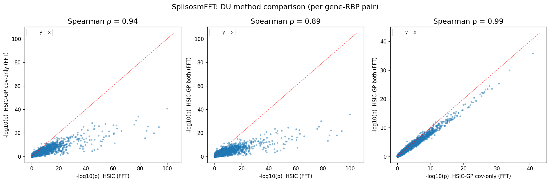
As expected, spatial conditioning mostly calibrates the p-values and reduces the number of significant hits, but the overall gene×factor pair rankings are highly correlated (Spearman’s rho = 0.89). Also, residualizing covariates only vs both covariates and probe usage ratios gives highly similar results (Spearman’s rho = 0.99), suggesting that the default approach is effective and robust.

pairs_fft = [
    ("pvalue_fft_hsic",    "pvalue_fft_gp_cov",
     "HSIC (FFT)",          "HSIC-GP cov-only (FFT)",  rho_h_gc),
    ("pvalue_fft_hsic",    "pvalue_fft_gp_both",
     "HSIC (FFT)",          "HSIC-GP both (FFT)",       rho_h_gb),
    ("pvalue_fft_gp_cov",  "pvalue_fft_gp_both",
     "HSIC-GP cov-only (FFT)", "HSIC-GP both (FFT)",   rho_gc_gb),
]

fig, axes = plt.subplots(1, 3, figsize=(15, 5))
for ax, (cx, cy, lx, ly, rho) in zip(axes, pairs_fft):
    x = _neg_log10(fft_all[cx].astype(float).values, floor=1e-100)
    y = _neg_log10(fft_all[cy].astype(float).values, floor=1e-100)
    ax.scatter(x, y, s=6, alpha=0.4, rasterized=True)
    lim = max(x.max(), y.max()) * 1.05
    ax.plot([0, lim], [0, lim], "r--", linewidth=1, alpha=0.6, label="y = x")
    ax.set_xlabel(f"-log10(p)  {lx}", fontsize=10)
    ax.set_ylabel(f"-log10(p)  {ly}", fontsize=10)
    ax.set_title(f"Spearman ρ = {rho:.2f}", fontsize=14)
    ax.legend(fontsize=8)

fig.suptitle("SplisosmFFT: DU method comparison (per gene-RBP pair)", fontsize=14)
fig.tight_layout()
plt.show()

Method comparison: SplisosmFFT vs SplisosmNP

Finally, let’s check the agreement between the FFT-accelerated SplisosmFFT and the original vectorized SplisosmNP implementations of the conditional DU test.

%%time
model_du_np = SplisosmNP()
model_du_np.setup_data(
    adata=sdata.tables['square_016um_svp'],
    design_mtx=sdata.tables['square_016um_rbp_sve'].layers['counts'],
    covariate_names=sdata.tables['square_016um_rbp_sve'].var[gene_name_col].values,
    spatial_key="spatial",
    layer="counts",
    group_iso_by=group_iso_by,
    gene_names=gene_name_col,
    min_counts=min_counts,
    min_bin_pct=min_bin_pct,
    filter_single_iso_genes=True,
    skip_spatial_kernel=True,  # spatial kernel construction not required for DU test
)
model_du_np

CPU times: user 84.2 ms, sys: 22 ms, total: 106 ms
Wall time: 110 ms

=== SplisosmNP
- Number of genes: 196
- Number of spots: 98917
- Number of covariates: 125
- Average isoforms per gene: 3.1
=== Model configurations
- Spatial kernel source: identity (skip_spatial_kernel=True)
- k_neighbors: N/A, rho: 0.99
- Standardize spatial covariance: True
=== Test results
- Spatial variability: N/A
- Differential usage: N/A

Run unconditional HSIC test with SplisosmNP

%%time
# Non-conditional: multivariate RV coefficient (no spatial residualization)
model_du_np.test_differential_usage(
    method="hsic",
    print_progress=True
)
du_np_hsic = model_du_np.get_formatted_test_results("du")
du_np_hsic = du_np_hsic.rename(columns={
    "pvalue": "pvalue_np_hsic",
    "statistic": "stat_np_hsic"
})
print(f"Significant DU (p<0.01, hsic): {(du_np_hsic['pvalue_np_hsic'] < 0.01).sum()}")

DU [hsic]: 100%|██████████| 196/196 [00:18<00:00, 10.32it/s]

Significant DU (p<0.01, hsic): 4075
CPU times: user 52 s, sys: 32 s, total: 1min 24s
Wall time: 21.8 s

Run conditional HSIC-GP test with SplisosmNP

For conditional DU on large irregular 2-D coordinates, use the NUFFT backend (requires the finufft package) to avoid a dense GP matrix. The speed-accuracy trade-off is controlled by lml_approx_rank, which tunes the eigensummary used for GP hyperparameter fitting; larger values are usually more accurate but use more memory and time.

%%time
model_du_np.test_differential_usage(
    method="hsic-gp", 
    residualize="cov_only",
    # run with NUFFT backend for better scalability
    # increase lml_approx_rank for better accuracy at the cost of speed
    gpr_backend="nufft",
    gpr_configs={"covariate": {"lml_approx_rank": 24}},
    # # The default sklearn backend uses subsampling for GP fitting
    # # increase n_inducing for better accuracy at the cost of speed
    # gpr_backend="sklearn",
    # gpr_configs={"covariate": {"n_inducing": 1000}},
    print_progress=True
)
du_np_gp_cov = model_du_np.get_formatted_test_results("du")
du_np_gp_cov = du_np_gp_cov.rename(columns={
    "pvalue": "pvalue_np_gp_cov",
    "statistic": "stat_np_gp_cov"
})
print(f"Significant DU (p<0.01, hsic-gp cov only): {(du_np_gp_cov['pvalue_np_gp_cov'] < 0.01).sum()}")

Covariates: 100%|██████████| 125/125 [01:44<00:00,  1.20it/s]
DU [hsic-gp]: 100%|██████████| 196/196 [00:15<00:00, 12.70it/s]

Significant DU (p<0.01, hsic-gp cov only): 3619
CPU times: user 2min 30s, sys: 49.9 s, total: 3min 20s
Wall time: 2min 1s

Compare conditional vs non-conditional test results, and SplisosmFFT vs SplisosmNP

def _neg_log10(p, floor=1e-300):
    return -np.log10(np.clip(p, floor, 1.0))

merge_cols = ["gene", "covariate"]

du_all = (
    du_fft_hsic[merge_cols + ["pvalue_fft_hsic"]]
    .merge(du_fft_gp_cov[merge_cols + ["pvalue_fft_gp_cov"]], on=merge_cols, how="inner")
    .merge(du_np_hsic[merge_cols + ["pvalue_np_hsic"]], on=merge_cols, how="inner")
    .merge(du_np_gp_cov[merge_cols + ["pvalue_np_gp_cov"]], on=merge_cols, how="inner")
)

# Spearman correlations between NP methods
rho_h_gc, _  = spearmanr(du_all["pvalue_np_hsic"],    du_all["pvalue_np_gp_cov"])
print(f"Spearman ρ(hsic vs hsic-gp[cov_only], SplisosmNP) = {rho_h_gc:.3f}")

# Spearman correlations between FFT and NP methods
rho_h, _  = spearmanr(du_all["pvalue_np_hsic"],    du_all["pvalue_fft_hsic"])
rho_gc, _ = spearmanr(du_all["pvalue_np_gp_cov"],  du_all["pvalue_fft_gp_cov"])
print(f"Spearman ρ(hsic, SplisosmNP vs SplisosmFFT) = {rho_h:.3f}")
print(f"Spearman ρ(hsic-gp[cov_only], SplisosmNP vs SplisosmFFT) = {rho_gc:.3f}")

Spearman ρ(hsic vs hsic-gp[cov_only], SplisosmNP) = 0.959
Spearman ρ(hsic, SplisosmNP vs SplisosmFFT) = 1.000
Spearman ρ(hsic-gp[cov_only], SplisosmNP vs SplisosmFFT) = 0.950

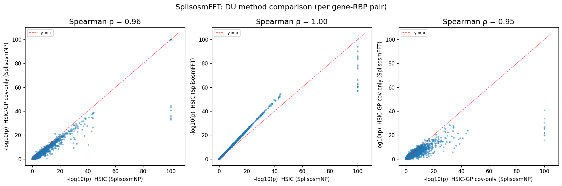
Due to rasterization (zero padding at unobserved bins), SplisosmFFT’s DU results will be slightly different from SplisosmNP’s, but the overall gene-factor pair rankings are still highly correlated.

pairs_du = [
    ("pvalue_np_hsic",    "pvalue_np_gp_cov",
     "HSIC (SplisosmNP)", "HSIC-GP cov-only (SplisosmNP)",  rho_h_gc),
    ("pvalue_np_hsic",    "pvalue_fft_hsic",
     "HSIC (SplisosmNP)", "HSIC (SplisosmFFT)",  rho_h),
    ("pvalue_np_gp_cov",  "pvalue_fft_gp_cov",
     "HSIC-GP cov-only (SplisosmNP)", "HSIC-GP cov-only (SplisosmFFT)",   rho_gc),
]

fig, axes = plt.subplots(1, 3, figsize=(15, 5))
for ax, (cx, cy, lx, ly, rho) in zip(axes, pairs_du):
    x = _neg_log10(du_all[cx].astype(float).values, floor=1e-100)
    y = _neg_log10(du_all[cy].astype(float).values, floor=1e-100)
    ax.scatter(x, y, s=6, alpha=0.4, rasterized=True)
    lim = max(x.max(), y.max()) * 1.05
    ax.plot([0, lim], [0, lim], "r--", linewidth=1, alpha=0.6, label="y = x")
    ax.set_xlabel(f"-log10(p)  {lx}", fontsize=10)
    ax.set_ylabel(f"-log10(p)  {ly}", fontsize=10)
    ax.set_title(f"Spearman ρ = {rho:.2f}", fontsize=14)
    ax.legend(fontsize=8)

fig.suptitle("SplisosmFFT: DU method comparison (per gene-RBP pair)", fontsize=14)
fig.tight_layout()
plt.show()

For reproducibility

import sys
from datetime import date
import splisosm

print("Last updated:", date.today())
print("Python:", sys.version.split()[0])
print("splisosm:", getattr(splisosm, "__version__", "unknown"))
print("spatialdata:", sd.__version__)

Last updated: 2026-05-03
Python: 3.12.13
splisosm: 1.2.0rc1
spatialdata: 0.7.2