Visium HD ONT (isoform)

This notebook demonstrates essential steps for analyzing spatial isoform usage using Visium HD with long-read (ONT) sequencing data:

1. Load preprocessed transcript-level quantification.

2. Run FFT-accelerated spatial variability tests with SplisosmFFT.

3. Compare results across spatial resolutions and with SplisosmNP.

For differential usage testing with SplisosmFFT, see the Visium HD FFPE (probe) Part II tutorial.

Estimated runtime: ~5 min.

Preliminary notes

In this tutorial, we use a Visium HD 3’ adult mouse brain (fresh frozen) data sequenced with Oxford Nanopore. For dataset access and workflow details, please check the official release page from EPI2ME.

Specifically, we downloaded the following outputs from the EPI2ME page:

- spaceranger/hac/HD_Adult_Mouse_Brain/
  # Space Ranger outputs (`possorted_genome_bam.bam` is not required).
- wf-single-cell/sup/SAMPLE_S1_L001/SAMPLE_S1_L001.transcript_raw_feature_bc_matrix_2um/
  # transcript-level count matrix (generated by EPI2ME with a custom pipeline).
- wf-single-cell/sup/SAMPLE_S1_L001/SAMPLE_S1_L001.transcriptome.gff.gz
  # GFF transcript annotation file.

We then ran convert_mtx_to_h5.py (available under the scripts directory) to prepare a barcode-by-transcript count matrix raw_tx_bc_matrix.h5, keeping only reference isoforms.

python convert_mtx_to_h5.py \
  './wf-single-cell/sup/SAMPLE_S1_L001/SAMPLE_S1_L001.transcript_raw_feature_bc_matrix_2um' \
  './wf-single-cell/sup/SAMPLE_S1_L001/SAMPLE_S1_L001.transcriptome.gff.gz' \
  'raw_tx_bc_matrix.h5'

Imports

from __future__ import annotations

import gzip
import re
import warnings
from pathlib import Path

import numpy as np
import pandas as pd
import matplotlib.pyplot as plt
from scipy.stats import spearmanr

import spatialdata as sd
import spatialdata_plot
from spatialdata import rasterize_bins

from splisosm import SplisosmFFT, SplisosmNP
from splisosm.utils import counts_to_ratios

warnings.filterwarnings("ignore", category=FutureWarning)
plt.rcParams["figure.dpi"] = 120
plt.rcParams["figure.figsize"] = (6, 4)

Configure paths and core parameters

# Input data (provided by user)
sdata_zarr = Path("/path/to/sdata_tx.filtered.zarr")
gff_file = Path("/path/to/SAMPLE_S1_L001.transcriptome.gff.gz")

# Resolution for primary testing
dataset_id = ""
test_table = "square_016um"
test_bins_element = f"{dataset_id}_{test_table}"

# Feature grouping and quality filters
group_iso_candidates = ["gene_ids", "gene_id"]
gene_name_candidates = ["gene_name", "gene_symbol", "gene_names"]

ONT data is generally more sparse than short-read data. To test as many genes as possible, we use a more lenient min_bin_pct threshold (the minimum percentage of non-zero bins required to keep an isoform).

# Isoform and gene filtering thresholds
min_counts = 10
min_bin_pct = 0.001 # a more lenient filter for sparse ONT data

Load preprocessed transcript-level SpatialData

We load the preprocessed SpatialData object generated by load_visiumhd_probe with raw_tx_bc_matrix.h5 as inputs.

%%time
if not sdata_zarr.exists(): 
    # from splisosm.io import load_visiumhd_probe
    # sdata = load_visiumhd_probe(
    #     path="./spaceranger/hac/HD_Adult_Mouse_Brain",
    #     bin_sizes=[2, 8, 16],
    #     filtered_counts_file=True,
    #     path_to_feature_2um_h5="raw_tx_bc_matrix.h5",
    # )
    # sdata.write_zarr("sdata_tx.filtered.zarr")
    raise FileNotFoundError(f"Cannot find Zarr store: {sdata_zarr}")
if not gff_file.exists():
    raise FileNotFoundError(f"Cannot find GFF file: {gff_file}")

print("Loading preprocessed SpatialData...")
sdata = sd.read_zarr(sdata_zarr)
sdata

Loading preprocessed SpatialData...
CPU times: user 7.06 s, sys: 1.09 s, total: 8.15 s
Wall time: 5.94 s

SpatialData object, with associated Zarr store: /Users/jysumac/Projects/SPLISOSM_paper/data/visiumhd_ont_mouse_cbs/sdata_tx.filtered.zarr
├── Images
│     ├── '_hires_image': DataArray[cyx] (3, 3000, 3200)
│     └── '_lowres_image': DataArray[cyx] (3, 563, 600)
├── Shapes
│     ├── '_square_002um': GeoDataFrame shape: (7857218, 1) (2D shapes)
│     ├── '_square_008um': GeoDataFrame shape: (492663, 1) (2D shapes)
│     └── '_square_016um': GeoDataFrame shape: (123658, 1) (2D shapes)
└── Tables
      ├── 'square_002um': AnnData (7857218, 48001)
      ├── 'square_008um': AnnData (492663, 48001)
      └── 'square_016um': AnnData (123658, 48001)
with coordinate systems:
    ▸ '', with elements:
        _hires_image (Images), _lowres_image (Images), _square_002um (Shapes), _square_008um (Shapes), _square_016um (Shapes)
    ▸ '_downscaled_hires', with elements:
        _hires_image (Images), _square_002um (Shapes), _square_008um (Shapes), _square_016um (Shapes)
    ▸ '_downscaled_lowres', with elements:
        _lowres_image (Images), _square_002um (Shapes), _square_008um (Shapes), _square_016um (Shapes)

Note that cell-segmentation results are not available for this dataset.

def pick_first(columns, candidates):
    for c in candidates:
        if c in columns:
            return c
    return None

print("Tables:", sorted(sdata.tables.keys()))
print("Images:", sorted(getattr(sdata, "images", {}).keys()))
print("Shapes:", sorted(getattr(sdata, "shapes", {}).keys()))

if test_table not in sdata.tables:
    raise ValueError(f"{test_table} is not available. Choose from: {sorted(sdata.tables.keys())}")

adata_test = sdata.tables[test_table]
group_iso_by = pick_first(adata_test.var.columns, group_iso_candidates)
if group_iso_by is None:
    raise ValueError(
        "Could not infer grouping column for transcript features. "
        f"Available var columns: {list(adata_test.var.columns)}"
    )

gene_name_col = pick_first(adata_test.var.columns, gene_name_candidates) or group_iso_by

if test_bins_element not in getattr(sdata, "shapes", {}):
    test_bins_element = test_table

print(f"Using table={test_table}, bins={test_bins_element}")
print(f"Grouping column={group_iso_by}, display names={gene_name_col}")

Tables: ['square_002um', 'square_008um', 'square_016um']
Images: ['_hires_image', '_lowres_image']
Shapes: ['_square_002um', '_square_008um', '_square_016um']
Using table=square_016um, bins=_square_016um
Grouping column=gene_ids, display names=gene_name

For each isoform, we have the following metadata columns (inferred from the GFF file):

adata_test.var.head(2)

	gene_ids	probe_ids	feature_types	gene_name	genome
ENSMUST00000000001	ENSMUSG00000000001	ENSMUST00000000001	Gene Expression	Gnai3
ENSMUST00000000028	ENSMUSG00000000028	ENSMUST00000000028	Gene Expression	Cdc45

As expected, the ONT-based data is sparser than short-read 3’ and targeted Visium HD datasets.

def summarize_table(adata):
    X = adata.layers["counts"] if "counts" in adata.layers else adata.X
    if hasattr(X, "nnz"):
        nnz = int(X.nnz)
        total = int(X.shape[0] * X.shape[1])
        density = nnz / total if total else np.nan
    else:
        arr = np.asarray(X)
        nnz = int(np.count_nonzero(arr))
        total = int(arr.size)
        density = nnz / total if total else np.nan
    return {
        "n_features": int(adata.n_vars),
        "n_bins": int(adata.n_obs),
        "count_mtx_density": density,
    }

rows = []
for key in sorted(sdata.tables.keys()):
    if key.startswith("square_"):
        rows.append({"table": key, **summarize_table(sdata.tables[key])})

pd.DataFrame(rows).sort_values("table")

	table	n_features	n_bins	count_mtx_density
0	square_002um	48001	7857218	0.000098
1	square_008um	48001	492663	0.001379
2	square_016um	48001	123658	0.004826

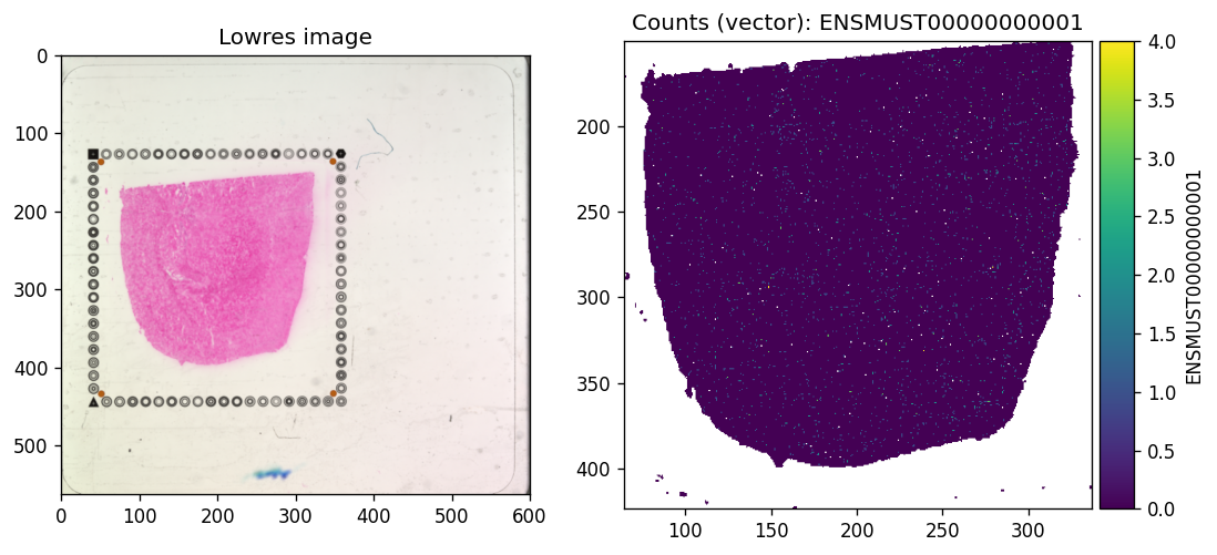
Finally, take a look at the tissue structure and spatial distribution of a few isoforms.

def ensure_rasterized(sdata, bin_table: str, bin_element: str, layer: str = "counts"):
    raster_key = f"rasterized_{bin_table}_{layer}"
    if raster_key in sdata.images:
        return raster_key

    adata = sdata.tables[bin_table]
    adata.X = adata.layers[layer] if layer in adata.layers else adata.X
    if hasattr(adata.X, "tocsc") and getattr(adata.X, "format", None) != "csc":
        adata.X = adata.X.tocsc()

    sdata[raster_key] = rasterize_bins(
        sdata,
        bins=bin_element,
        table_name=bin_table,
        col_key="array_col",
        row_key="array_row",
    )
    return raster_key

%%time
tx_name = 'ENSMUST00000000001' # Gnai3
axes = plt.subplots(1, 2, figsize=(10, 5))[1].flatten()
sdata.pl.render_images(f"{dataset_id}_lowres_image").pl.show(
    coordinate_systems=f"{dataset_id}_downscaled_lowres",
    ax=axes[0], title="Lowres image"
)
sdata.pl.render_shapes(f"{dataset_id}_square_016um", color=tx_name).pl.show(
    coordinate_systems=f"{dataset_id}_downscaled_lowres",
    ax=axes[1], title=f"Counts (vector): {tx_name}"
)

CPU times: user 6.38 s, sys: 791 ms, total: 7.17 s
Wall time: 7.32 s

Spatial variability testing with SplisosmFFT

model = SplisosmFFT(neighbor_degree=1, rho=0.99)
model.setup_data(
    sdata=sdata,
    bins=test_bins_element,
    table_name=test_table,
    col_key="array_col",
    row_key="array_row",
    layer="counts",
    group_iso_by=group_iso_by,
    gene_names=gene_name_col,
    min_counts=min_counts,
    min_bin_pct=min_bin_pct,
    filter_single_iso_genes=True
)
model

=== SplisosmFFT
- Number of genes: 1558
- Number of spots: 123658
- Number of spots after rasterization: 175561
- Number of covariates: 0
- Average isoforms per gene: 2.3
=== Model configurations
- Neighborhood degree: 1
- Spatial autocorrelation rho: 0.99
=== Test results
- Spatial variability: N/A
- Differential usage: N/A

While many genes have more than 10 isoforms detected, the effective number of isoforms (adjusted for expression level) is much smaller.

%%time
gene_meta = model.extract_feature_summary(level="gene")
feature_meta = model.extract_feature_summary(level="isoform")
gene_meta.sort_values("perplexity", ascending=False).head(5)

Genes: 100%|██████████| 1558/1558 [00:00<00:00, 1937.07it/s]

CPU times: user 813 ms, sys: 146 ms, total: 959 ms
Wall time: 962 ms

	n_isos	perplexity	pct_bin_on	count_avg	count_std	major_ratio_avg
gene
Pantr1	9	7.620990	0.024964	0.032291	0.221045	0.229902
Mtch1	8	7.095370	0.023144	0.029185	0.205137	0.234968
Gas5	17	6.323551	0.111630	0.165667	0.564609	0.476765
Egfl7	6	5.437132	0.014726	0.018689	0.165910	0.272177
Paxx	7	5.433822	0.035930	0.048642	0.276595	0.321363

Next, we run method="hsic-ir" to detect spatial variability in isoform usage.

%%time
model.test_spatial_variability(
    method="hsic-ir",
    ratio_transformation="none",
    n_jobs=-1,
    print_progress=True,
)

SV [hsic-ir]: 100%|██████████| 116/116 [00:04<00:00, 23.42it/s]

CPU times: user 24.5 s, sys: 5.28 s, total: 29.8 s
Wall time: 6.33 s

sv_res_16um = model.get_formatted_test_results(
    "sv", with_gene_summary=True
).sort_values("pvalue_adj")
sv_res_16um.head(5)

	gene	statistic	pvalue	pvalue_adj	n_isos	perplexity	pct_bin_on	count_avg	count_std	major_ratio_avg
1133	Nnat	3.349203e-07	0.0	0.0	2	1.650491	0.073922	0.113628	0.503994	0.799516
1356	Gls	6.044231e-07	0.0	0.0	2	1.460988	0.170721	0.241117	0.614752	0.873793
340	Caly	4.102586e-07	0.0	0.0	4	2.824695	0.052330	0.071544	0.337891	0.579632
610	Fxyd1	2.116209e-07	0.0	0.0	5	3.250710	0.031886	0.043297	0.265310	0.555099
1218	Olfm1	7.099970e-07	0.0	0.0	3	2.023517	0.177611	0.269962	0.701330	0.766378

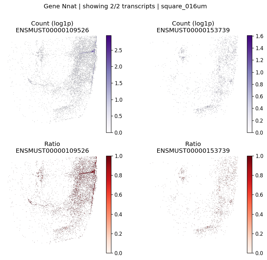
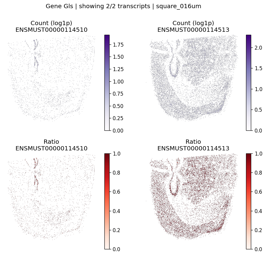
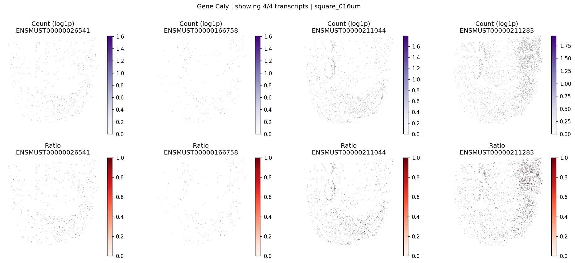
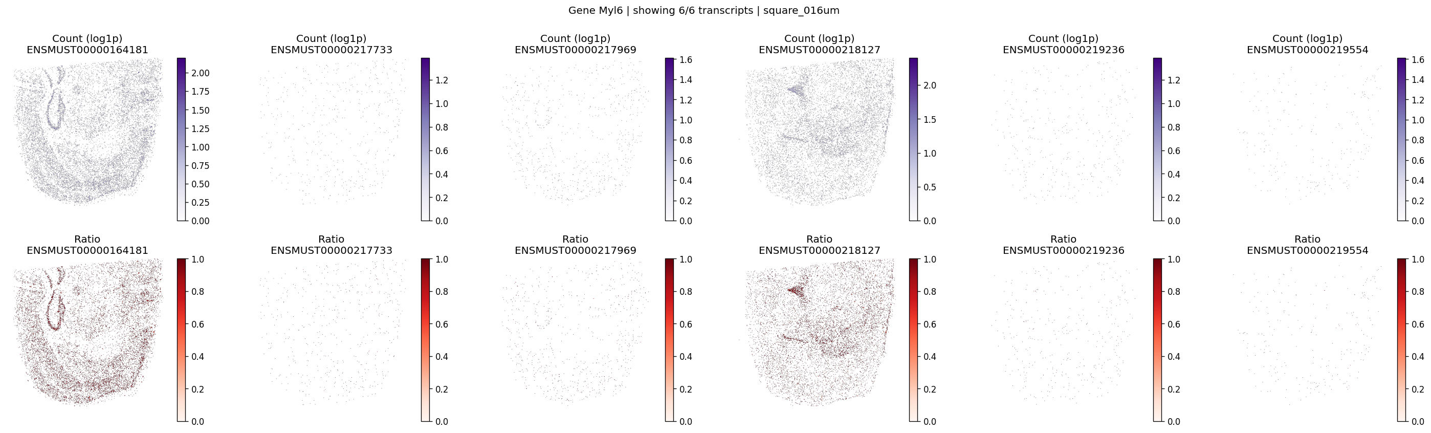
Let’s take a look at the top significant genes and their spatial isoform usage patterns.

sig_001 = int((sv_res_16um["pvalue_adj"] < 0.01).sum())
print(
    "Spatially variable genes (FDR < 0.01, 16 µm): "
    f"{sig_001} out of {sv_res_16um.shape[0]} total genes"
)
top_genes = sv_res_16um.head(10)["gene"].astype(str).tolist()
top_genes[:5]

Spatially variable genes (FDR < 0.01, 16 µm): 710 out of 1558 total genes

['Nnat', 'Gls', 'Caly', 'Fxyd1', 'Olfm1']

Show code cell source

Hide code cell source

def plot_gene_tx_maps(
    sdata,
    bin_table: str,
    bin_element: str,
    gene_id: str,
    tx_meta: pd.DataFrame | None = None,
    group_col: str = "gene_ids",
    max_peaks: int = 4,
    hide_zero_count: bool = True,
    hide_zero_ratio: bool = True,
):
    adata = sdata.tables[bin_table]
    if tx_meta is None:
        tx_meta = adata.var.copy()

    if group_col not in tx_meta.columns:
        raise ValueError(f"'{group_col}' not found in tx_meta columns")

    tx_names = tx_meta.index[
        tx_meta[group_col].astype(str) == str(gene_id)
    ].tolist()
    if len(tx_names) == 0:
        raise ValueError(f"No transcripts found for gene id '{gene_id}'")
    if any(tx not in adata.var_names for tx in tx_names):
        raise ValueError(f"Some transcripts not found in {bin_table}.var_names")
    n_peaks = len(tx_names)
    n_shown = min(n_peaks, max_peaks)
    tx_names = tx_names[:n_shown]

    raster_key = ensure_rasterized(sdata, bin_table=bin_table, bin_element=bin_element)
    data = sdata[raster_key].sel(c=tx_names).values
    counts_cube = np.moveaxis(np.asarray(data, dtype=float), 0, -1)

    counts_flat = counts_cube.reshape(-1, counts_cube.shape[-1])
    ratios_flat = counts_to_ratios(counts_flat, transformation="none", nan_filling="none")
    ratios_cube = ratios_flat.numpy().reshape(counts_cube.shape)

    n_tx = counts_cube.shape[-1]
    fig, axes = plt.subplots(2, n_tx, figsize=(4 * n_tx, 7), squeeze=False)

    for i, tx in enumerate(tx_names):
        c = counts_cube[:, :, i]
        r = ratios_cube[:, :, i]
        if hide_zero_count:
            c = np.where(c == 0, np.nan, c)
        if hide_zero_ratio:
            r = np.where(r == 0, np.nan, r)

        im0 = axes[0, i].imshow(np.log1p(c), cmap="Purples", vmin=0.0)
        axes[0, i].set_title(f"Count (log1p)\n{tx}")
        axes[0, i].axis("off")
        fig.colorbar(im0, ax=axes[0, i], fraction=0.046, pad=0.04)

        vmax = np.nanpercentile(ratios_cube, 99) if np.isfinite(ratios_cube).any() else 1.0
        im1 = axes[1, i].imshow(r, cmap="Reds", vmin=0.0, vmax=vmax)
        axes[1, i].set_title(f"Ratio\n{tx}")
        axes[1, i].axis("off")
        fig.colorbar(im1, ax=axes[1, i], fraction=0.046, pad=0.04)

    fig.suptitle(f"Gene {gene_id} | showing {n_shown}/{n_peaks} transcripts | {bin_table}", y=1)
    fig.tight_layout()
    plt.show()

# Visualize maps for a few significant genes
for gene_id in top_genes[:3]:
    plot_gene_tx_maps(
        sdata=sdata,
        bin_table=test_table,
        bin_element=test_bins_element,
        gene_id=gene_id,
        tx_meta=feature_meta,
        group_col='gene_name',
        max_peaks=6,
        hide_zero_ratio=True,
    )

%%time
# Plot an example gene of interest
plot_gene_tx_maps(
    sdata=sdata,
    bin_table=test_table,
    bin_element=test_bins_element,
    gene_id='Myl6',
    tx_meta=feature_meta,
    group_col='gene_name',
    max_peaks=6,
    hide_zero_ratio=True,
)

CPU times: user 401 ms, sys: 40.9 ms, total: 442 ms
Wall time: 445 ms

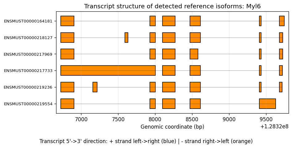
And the transcript structure of a gene (showing kept isoforms after filtering):

Show code cell source

Hide code cell source

def _open_text(path: Path):
    if str(path).endswith(".gz"):
        return gzip.open(path, "rt")
    return open(path, "rt")


def _extract_attr(attr_text: str, key: str) -> str | None:
    m = re.search(rf"{re.escape(key)}[= ]\"?([^\";]+)", str(attr_text))
    return m.group(1) if m else None


def _normalize_tx_id(value: str) -> str:
    token = str(value).strip().split("|")[0].split(";")[0].split(" ")[0]
    # Strip Ensembl transcript version only (e.g. ENSMUST....1.2 -> ENSMUST....1)
    m = re.match(r"^(ENSMUST\d+)\.\d+$", token)
    if m:
        return m.group(1)
    return token


def _build_reference_tx_structures(gff_path: Path) -> dict[str, list[dict]]:
    """Build exon structures keyed by reference transcript ID (cmp_ref/ENSMUST)."""
    assembled_meta: dict[str, dict] = {}
    assembled_exons: dict[str, list[tuple[int, int]]] = {}

    with _open_text(gff_path) as f:
        for line in f:
            if line.startswith("#"):
                continue
            parts = line.rstrip("\n").split("\t")
            if len(parts) < 9:
                continue

            feature_type = parts[2].lower()
            attr = parts[8]

            if feature_type in {"transcript", "mrna"}:
                tx_id = _extract_attr(attr, "transcript_id") or _extract_attr(attr, "ID")
                if not tx_id:
                    continue

                cmp_ref = _extract_attr(attr, "cmp_ref")
                ref_tx_id = _normalize_tx_id(cmp_ref) if cmp_ref else _normalize_tx_id(tx_id)

                assembled_meta[tx_id] = {
                    "assembled_tx_id": tx_id,
                    "ref_tx_id": ref_tx_id,
                    "chrom": parts[0],
                    "strand": parts[6],
                    "class_code": _extract_attr(attr, "class_code") or "",
                    "gene_id": _extract_attr(attr, "ref_gene_id")
                    or _extract_attr(attr, "gene_id")
                    or "",
                    "gene_name": _extract_attr(attr, "ref_gene_name")
                    or _extract_attr(attr, "gene_name")
                    or _extract_attr(attr, "cmp_ref_gene")
                    or "",
                }

            elif feature_type == "exon":
                tx_id = (
                    _extract_attr(attr, "transcript_id")
                    or _extract_attr(attr, "Parent")
                    or _extract_attr(attr, "ID")
                )
                if not tx_id:
                    continue
                assembled_exons.setdefault(tx_id, []).append((int(parts[3]), int(parts[4])))

    ref_to_structs: dict[str, list[dict]] = {}
    for tx_id, meta in assembled_meta.items():
        exons = sorted(assembled_exons.get(tx_id, []))
        if len(exons) == 0:
            continue

        structure = {
            **meta,
            "exons": exons,
            "start": min(e[0] for e in exons),
            "end": max(e[1] for e in exons),
            "n_exons": len(exons),
            "tx_len": sum((e2 - e1) for e1, e2 in exons),
        }
        ref_to_structs.setdefault(meta["ref_tx_id"], []).append(structure)

    return ref_to_structs


def _pick_best_structure(candidates: list[dict]) -> dict:
    """Pick one representative structure per reference transcript."""
    class_rank = {
        "=": 6,
        "k": 5,
        "j": 4,
        "c": 3,
        "i": 2,
        "o": 1,
        "u": 0,
    }

    def _score(c: dict) -> tuple[int, int, int]:
        return (
            class_rank.get(str(c.get("class_code", "")).strip(), -1),
            int(c.get("n_exons", 0)),
            int(c.get("tx_len", 0)),
        )

    return sorted(candidates, key=_score, reverse=True)[0]


def plot_feature_transcript_structure(
    sdata,
    bin_table: str,
    gene_id: str,
    feature_meta: pd.DataFrame,
    group_col: str,
    gff_path: str | Path,
    top_k: int = 8,
    figsize: tuple[float, float] = (8, 4),
):
    """Plot exon structures for reference transcripts selected from feature_meta."""
    adata = sdata.tables[bin_table]
    gff_path = Path(gff_path)

    # 1) Get transcripts for this gene from feature_meta
    gene_mask = feature_meta[group_col].astype(str) == str(gene_id)

    gene_features = feature_meta.loc[gene_mask].copy()
    if gene_features.empty:
        raise ValueError(f"No features found for gene '{gene_id}'")

    feature_names = gene_features.index.tolist()
    x_sub = adata[:, feature_names].layers.get("counts", adata[:, feature_names].X)
    feature_sums = np.asarray(x_sub.sum(axis=0)).ravel()
    order = np.argsort(-feature_sums)

    ref_tx_ids = []
    seen = set()
    for i in order:
        tx = _normalize_tx_id(feature_names[i])
        if tx not in seen:
            ref_tx_ids.append(tx)
            seen.add(tx)
        if len(ref_tx_ids) >= top_k:
            break

    # 2) Query GFF structures by reference transcript ID (via cmp_ref)
    ref_to_structs = _build_reference_tx_structures(gff_path)

    resolved: list[tuple[str, dict]] = []
    missing: list[str] = []
    for ref_tx in ref_tx_ids:
        candidates = ref_to_structs.get(ref_tx, [])
        if len(candidates) == 0:
            missing.append(ref_tx)
            continue
        resolved.append((ref_tx, _pick_best_structure(candidates)))

    if len(resolved) == 0:
        examples = ", ".join(ref_tx_ids[:5])
        raise ValueError(
            "Could not find transcript exon structures in GFF for selected reference transcripts. "
            f"Example IDs: {examples}."
        )

    # 3) Plot exon structures, labeled by reference transcript ID
    fig, ax = plt.subplots(figsize=figsize)
    strand_colors = {"+": "steelblue", "-": "darkorange"}

    y_positions = np.arange(len(resolved))
    x_mins: list[int] = []
    x_maxs: list[int] = []

    for y, (ref_tx, info) in zip(y_positions, resolved, strict=False):
        tx_min, tx_max = int(info["start"]), int(info["end"])
        x_mins.append(tx_min)
        x_maxs.append(tx_max)

        tx_color = strand_colors.get(str(info.get("strand", ".")), "gray")
        ax.plot([tx_min, tx_max], [y, y], color="black", linewidth=0.5, alpha=0.5)

        for exon_start, exon_end in info["exons"]:
            ax.barh(
                y,
                exon_end - exon_start,
                left=exon_start,
                height=0.6,
                color=tx_color,
                edgecolor="black",
            )

    ax.set_yticks(y_positions)
    ax.set_yticklabels([ref_tx for ref_tx, _ in resolved], fontsize=8)
    ax.invert_yaxis()
    ax.set_xlabel("Genomic coordinate (bp)")
    ax.set_title(f"Transcript structure of detected reference isoforms: {gene_id}")
    ax.grid(True, axis="x", alpha=0.3)

    if x_mins and x_maxs:
        x_pad = (max(x_maxs) - min(x_mins)) * 0.02
        if x_pad > 0:
            ax.set_xlim(min(x_mins) - x_pad, max(x_maxs) + x_pad)

    direction_note = "Transcript 5'->3' direction: + strand left->right (blue) | - strand right->left (orange)"
    fig.text(0.5, 0.01, direction_note, ha="center", va="bottom", fontsize=10, color="black")

    if missing:
        note = f"Missing in GFF: {', '.join(missing[:4])}" + (" ..." if len(missing) > 4 else "")
        fig.text(0.5, 0.035, note, ha="center", va="bottom", fontsize=8, color="dimgray")

    fig.tight_layout(rect=(0.0, 0.07, 1.0, 1.0))
    plt.show()

%%time
# Plot an example gene of interest with transcript structures
plot_feature_transcript_structure(
    sdata=sdata,
    bin_table=test_table,
    gene_id="Myl6",
    feature_meta=feature_meta,
    group_col="gene_name",
    gff_path=gff_file,
    top_k=10,
)

CPU times: user 2.84 s, sys: 51.6 ms, total: 2.89 s
Wall time: 2.9 s

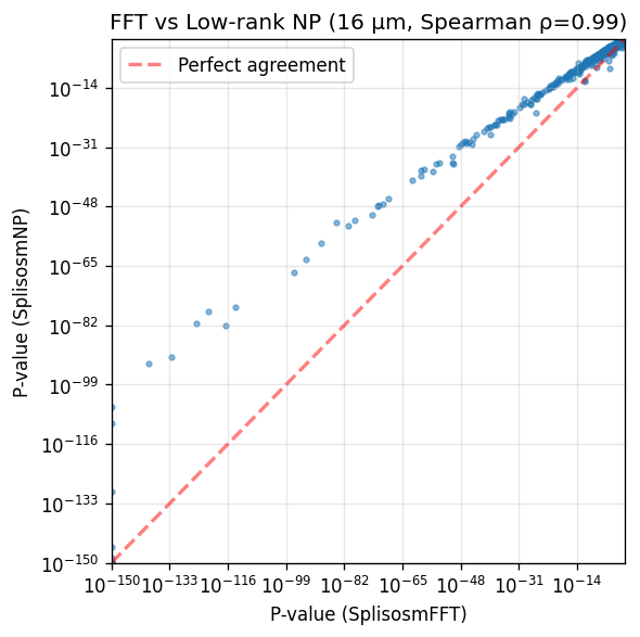
Method comparison: SplisosmFFT vs SplisosmNP

We now compare FFT-accelerated and non-parametric spatial variability tests at 16 µm resolution.

Note: Since v1.2.0, SplisosmNP SV tests use Liu’s approximation from full-rank spatial-kernel cumulants by default. See the SV hyperparameter optimization notebook for comparison with the legacy low-rank approach.

For large implicit CAR kernels, null_configs={"n_probes": m} controls the Hutchinson trace budget. Smaller m is faster but noisier. To emphasize broad smooth patterns, prefer increasing rho (for example, rho=0.999) rather than rank truncation.

%%time
# Run SplisosmNP at 16µm for direct comparison with SplisosmFFT
model_np = SplisosmNP(
    k_neighbors=4,
    rho=0.99,
    standardize_cov=False # faster
)
model_np.setup_data(
    adata=sdata.tables[test_table],
    spatial_key='spatial', # adata.obsm key for spatial coordinates
    layer='counts',
    group_iso_by=group_iso_by, # 'gene_ids'
    gene_names=gene_name_col, # 'gene_ids'
    min_counts=min_counts,
    min_bin_pct=min_bin_pct,
    min_component_size=10 # remove disconnected tissue fragments if any
)

/Users/jysumac/Projects/SPLISOSM/src/splisosm/utils/preprocessing.py:832: UserWarning: Removed 100 spot(s) belonging to graph components with fewer than 10 member(s). 123558 spot(s) remain.
  spatial_inputs = _filter_small_components(

CPU times: user 508 ms, sys: 103 ms, total: 611 ms
Wall time: 616 ms

%%time
model_np.test_spatial_variability(
    method='hsic-ir',
    null_configs={"n_probes": 60},
    ratio_transformation='none',
    print_progress=True,
)

SV [hsic-ir]: 100%|██████████| 116/116 [00:03<00:00, 33.01it/s]

CPU times: user 29.9 s, sys: 3.07 s, total: 33 s
Wall time: 5.26 s

Compare p-values between SplisosmFFT and SplisosmNP:

# Extract results and merge
sv_np = model_np.get_formatted_test_results('sv')[['gene', 'pvalue']].copy()
sv_np = sv_np.rename(columns={'pvalue': 'pvalue_np'})

comparison = sv_res_16um[['gene', 'pvalue']].copy()
comparison = comparison.rename(columns={'pvalue': 'pvalue_fft'})
comparison = comparison.merge(sv_np, on='gene', how='inner')

corr, _ = spearmanr(comparison['pvalue_fft'], comparison['pvalue_np'])

print(f'Genes tested in both methods: {len(comparison)}')
print(f'== Significant in SplisosmFFT (FDR < 0.01): {(comparison["pvalue_fft"] < 0.01).sum()}')
print(f'== Significant in SplisosmNP (FDR < 0.01): {(comparison["pvalue_np"] < 0.01).sum()}')
print(f'== P-value correlation (Spearman rho): {corr:.4f}')

Genes tested in both methods: 1558
== Significant in SplisosmFFT (FDR < 0.01): 790
== Significant in SplisosmNP (FDR < 0.01): 538
== P-value correlation (Spearman rho): 0.9903

The two approaches yield almost identical rankings. SplisosmFFT shows slightly smaller p-values for top genes due to zero-padding that increases sample size (n=123,658 before vs n=175,561 after rasterization).

# Scatter plot comparison
fig, ax = plt.subplots(figsize=(5, 5))
x = comparison['pvalue_fft'].to_numpy()
y = comparison['pvalue_np'].to_numpy()

ax.scatter(x + 1e-150, y + 1e-150, s=8, alpha=0.5)
ax.set_xscale('log')
ax.set_yscale('log')
ax.set_xlabel('P-value (SplisosmFFT)')
ax.set_ylabel('P-value (SplisosmNP)')
ax.set_title(f'FFT vs Low-rank NP (16 µm, Spearman ρ={corr:.2f})')
ax.grid(True, alpha=0.3)

# Add diagonal reference line
lims = [1e-150, 1.0]
ax.plot(lims, lims, 'r--', alpha=0.5, label='Perfect agreement', linewidth=2)
ax.legend()
ax.set_xlim(lims)
ax.set_ylim(lims)

plt.tight_layout()
plt.show()

For reproducibility

import sys
from datetime import date
import splisosm

print("Last updated:", date.today())
print("Python:", sys.version.split()[0])
print("splisosm:", getattr(splisosm, "__version__", "unknown"))

Last updated: 2026-05-03
Python: 3.12.13
splisosm: 1.2.0rc1