Frequently Asked Questions#
Installation#
Please report any installation issues on the GitHub Issues page.
Platform compatibility#
1. Which spatial transcriptomics platforms are supported by SPLISOSM?
SPLISOSM is designed to be platform-agnostic and can be applied to data from any spatial transcriptomics technology, as long as isoform-level quantification is available. We have confirmed that the following platforms generate data that can be directly analyzed by SPLISOSM:
Short-read: 10x Visium (FFPE, 3’), 10x Visium HD (FFPE, 3’), Slide-seqV2.
Long-read: 10x Visium ONT, 10x Visium HD ONT.
In situ: 10x Xenium Prime 5K.
See the Feature Quantification page for guidance on preparing input data from different platforms, and the Tutorial Gallery for example analyses.
2. I am not interested in isoform-level analysis. Can I use SPLISOSM for gene-level spatial variability testing?
Yes. The gene-level spatial variability test, HSIC-GC, is also available as a standalone function,
splisosm.utils.stats.run_hsic_gc(). It can be used as a drop-in replacement for other spatial gene expression analysis tools like SPARK-X.from splisosm.utils.stats import run_hsic_gc import numpy as np # ── matrix mode ────────────────────────────────────────────────── # gene expression matrix: (n_spot, n_gene) gene_counts = np.random.randn(100, 50) # spatial coordinates: (n_spot, 2) coordinates = np.random.rand(100, 2) # run HSIC-GC test (default: Liu's cumulant approximation for the null) # null_configs={"n_probes": m} controls the Hutchinson probe budget # Default is 60. Use a smaller m for faster computation test_results = run_hsic_gc(gene_counts, coordinates, n_jobs=-1) print(test_results['statistic']) # test statistics, (n_gene,) print(test_results['pvalue']) # p-values, (n_gene,) # ── AnnData mode ───────────────────────────────────────────────── # adata.X or adata.layers[layer] must be a (n_spots, n_genes) count # matrix (dense or scipy sparse); adata.obsm[spatial_key] provides # spatial coordinates. test_results = run_hsic_gc( adata=adata, # AnnData of shape (n_spots, n_genes) layer=None, # None → use adata.X; str → use adata.layers[layer] spatial_key="spatial", min_counts=1, # optional: drop genes with fewer total counts min_bin_pct=0.05, # optional: drop genes expressed in < 5% of spots n_jobs=-1, # optional: parallelize gene chunks )
Choosing a model class#
3. What is the difference between SplisosmNP, SplisosmFFT, and SplisosmGLMM?
SPLISOSM provides three model classes, each targeting a different use case:
SplisosmNP— non-parametric HSIC tests using a sparse CAR spatial kernel. Supports both SV and DU testing, works on arbitrary geometries (irregular spots, single cells, segmented tissue), and acceptsAnnDatainput. Recommended default for most datasets.
SplisosmFFT— FFT-accelerated HSIC tests on regular grids (Visium HD, Xenium binned data). Shares the same statistical model asSplisosmNPbut exploits the translation invariance of regular lattices to perform convolutions in Fourier space. Accepts aSpatialDataobject as input. Recommended for large regular-grid datasets for fast computation and lower memory footprint.
SplisosmGLMM— parametric multinomial GLMM with a Gaussian random field spatial random effect. Supports DU testing only. Potentially more interpretable (effect sizes, confidence intervals etc.) but requires fitting a model per gene, which is computationally intensive. Use when you need effect-size estimates.See Quick Start for a model-selection decision tree.
4. Why do SplisosmNP and SplisosmFFT give different results?
While sharing the same statistical methodology, p-values from the two classes can differ for three reasons:
1. Periodic boundary assumption.
SplisosmFFTtreats the grid as periodic (block-circulant kernel), which means bins at opposite edges of the grid are treated as spatial neighbours. In contrast,SplisosmNPbuilds a k-NN graph from the actual coordinates and has no wrap-around. The boundary effect is usually small when tissue occupies the interior of a larger zero-padded grid.2. Rasterisation and zero-padding.
SplisosmFFToperates on the full \(H \times W\) raster grid. Unobserved bins (positions absent in thesdata.tablesAnnData) are zero-padded (as if they had zero counts).SplisosmNPoperates only on the \(n \le H \times W\) observed spots recorded in the AnnData, so the effective sample size and kernel matrix dimensions can differ.3. SplisosmNP large-kernel null approximation. For large implicit CAR kernels,
SplisosmNPestimates Liu null cumulants with Hutchinson Rademacher probes by default, which can lead to slightly different p-values compared to a full eigendecomposition. The shared probe budget is controlled vianull_configs={"n_probes": m}for both Liu cumulants and Welch trace probes.In practice, when the grid is densely observed (few missing bins) and the tissue is far from the grid boundary, the two classes give very similar results. Low-rank approximation is no longer needed for
SplisosmNPSV tests because the default Liu path works from direct cumulants rather than the full pairwise eigenvalue product.
5. Why did SplisosmNP SV results change in v1.2.0?
Starting in v1.2.0,
SplisosmNPuses Liu’s approximation with full-rank spatial-kernel cumulants by default. In v1.1.x, largeSplisosmNPSV tests used a low-rank spatial approximation by default. This can change p-values and the number of SVP genes passing a fixed FDR threshold, although gene rankings are usually largely consistent.At first glance, the legacy low-rank approach may appear to have higher statistical power because it often identifies more SVP genes. This happens because low-rank approximations keep broad, low-frequency spatial patterns and drop finer local variation. Since real spatial datasets often contain strong global patterns, the low-rank test can naturally produce smaller p-values in those scenarios.
For applications that intentionally prioritize global patterns, prefer adjusting the spatial kernel instead of returning to rank truncation; for example, use a smoother CAR kernel such as
SplisosmNP(rho=0.999)orrun_hsic_gc(..., rho=0.999). This keeps the full-rank test able to detect local patterns while increasing emphasis on global smooth structure. Usenull_configs={"n_probes": m}only to tune the stochastic cumulant trace budget; it is not a low-rank approximation. See the Visium HD SV hyperparameter tutorial for a benchmark comparing FFT, full-rank NP, smoother full-rank NP, and the legacy low-rank diagnostic path.
6. Which differential usage test method should I use: parametric or non-parametric?
We recommend using the non-parametric test (
SplisosmNPwithmethod='hsic-gp') as the default choice. It is more robust to model misspecification and generally provides better control of the false positive rate. The parametric test (SplisosmGLMM) allows for the inclusion of covariates and confounders, which can be useful in specific experimental designs.Note that both conditional tests (
'hsic-gp'and'glmm') are computationally intensive and may take hours to run on large datasets. For'hsic-gp', irregular 2-D coordinates can use the FINUFFT-backedgpr_backend="nufft"path to avoid dense GP matrices. The sklearn and gpytorch backends also support subset or inducing-point controls vian_inducing. See GP Regression Backends for backend-specific options. For'glmm', model fitting is handled natively with PyTorch with GPU device support, and low-rank kernel approximation is also available (viaSplisosmGLMM(approx_rank=...)).from splisosm import SplisosmNP model_np = SplisosmNP() model_np.setup_data(...) model_np.test_differential_usage( method="hsic-gp", residualize="cov_only", # recommended for large irregular 2-D data gpr_backend="nufft", gpr_configs={"covariate": {"lml_approx_rank": 64}}, )Alternatively, consider the faster unconditional tests (
'hsic'or'glm'). While they do not account for spatial autocorrelation and may be anti-conservative (inflated false-positive rate), the overall ranking of gene-covariate associations is often similar to the conditional tests, especially for top hits.from splisosm import SplisosmGLMM, SplisosmNP # non-parametric DU test (unconditional) model_np = SplisosmNP() model_np.setup_data(...) # the unconditional test is equivalent to the multivariate correlation coefficient test model_np.test_differential_usage(method='hsic') # parametric DU test using GLM (unconditional) model_glm = SplisosmGLMM(model_type='glm') model_glm.setup_data(...) model_glm.fit() model_glm.test_differential_usage(method='score')
Running SPLISOSM#
7. Can I run SPLISOSM on single-cell spatial transcriptomics data?
Yes.
SplisosmNPworks directly on segmented single-cell data — simply pass the cell-level AnnData with spatial coordinates. See the Xenium segmented single-cell tutorial for a worked example, and the Feature Quantification page for guidance on preparing input data from Space Ranger and Xenium Ranger segmentation outputs.
8. Can I run SPLISOSM on a subset of cells/spots instead of the whole tissue?
Yes. SPLISOSM can be run on any subset of cells or spots. This is useful when focusing on specific regions of interest or cell types. Simply filter your AnnData object to the subset of interest before passing it to SPLISOSM. See the Xenium segmented single-cell tutorial for an example.
If your selection consists of disconnected regions, the spatial relationships might be distorted. To preserve the original global spatial context, you can use the full dataset to build the spatial kernel. A simple way to achieve this is to prepare an input matrix containing all spots but set the isoform counts for unselected spots to zero. SPLISOSM will then ignore these spots in the statistical tests while still using their coordinates to build the spatial kernel.
9. Can I run SPLISOSM on single-cell non-spatial transcriptomics data?
Yes. While SPLISOSM is designed to identify patterns associated with physical spatial coordinates, it is technically possible to run it on non-spatial single-cell RNA-seq data. This can be done by treating cell embeddings (e.g., PCA or UMAP coordinates) as “pseudo-spatial coordinates.”
SplisosmNPnatively supports high-dimensional coordinate arrays (any number of dimensions ≥ 2). Simply pass the PCA embedding matrix as thespatial_key(or a pre-computed graph adjacency matrix, such asadata.obsp['connectivities']as theadj_key) insetup_data. Note that the conditional differential usage testmethod='hsic-gp'requires coordinates fromspatial_keyto fit Gaussian Process models, even ifadj_keyis provided. See the final section of the Xenium segmented single-cell tutorial for an example.This approach should be used with caution: ‘spatial’ patterns in this case are only as meaningful as the biological relationships captured by the embedding. Furthermore, be aware of potential circularity if the isoform data was used to generate the embeddings, as this may lead to spurious associations.
Interpretation of Results#
10. For genes with spatially variable RNA processing (SVP), can I tell which isoforms are driving the spatial variability?
Yes and no. Isoform usage ratios are compositional, meaning they sum to one for each gene in a given spot or cell. If one isoform’s usage increases in a spatial region, the usage of one or more other isoforms must decrease. For this reason, SPLISOSM’s primary differential usage test (HSIC-IR) is a gene-level multivariate test that aggregates signals across all of a gene’s isoforms.
However, for genes with more than two isoforms, it is possible to rank the isoforms by their individual contributions to the overall spatial pattern. This can be done by computing a separate univariate spatial variability statistic (e.g., HSIC) for each isoform’s usage ratio.
from splisosm.utils.preprocessing import counts_to_ratios
from splisosm.utils.stats import run_hsic_gc
import numpy as np

# example data
data = np.random.rand(100, 3)  # (n_spot, n_iso), isoform expression matrix for a gene with 3 isoforms
data[data < 0] = 0  # ensure non-negative values

# compute isoform ratios
data = counts_to_ratios(data, transformation='none', nan_filling='mean') # (n_spot, n_iso)
coordinates = np.random.rand(100, 2)  # (n_spot, 2), spatial coordinates

# compute per-isoform univariate HSIC test using HSIC-GC
sv_results = run_hsic_gc(data, coordinates) # dict with 'statistic' and 'pvalue' for each isoform

# rank isoforms by their HSIC test results
ranked_isoform_indices = np.argsort(sv_results['pvalue'])  # ascending order
Note
This per-isoform ranking is for exploratory purposes only. The adjusted p-values from this analysis should not be considered as formal hypothesis testing, as the usage ratios of isoforms from the same gene are inherently correlated.
11. How many spatially variably expressed (SVE) genes or spatially variably processed (SVP) genes should I expect to find?
The number of detected SVE/SVP genes depends on many factors, including the biological system, data quality, and sequencing depth. For example, in our analyses of the adult mouse brain (Visium + ONT and Visium 3’), the number of detected SVP genes did not saturate at the sequencing depths tested. We observed that the number of detected SVP genes increased linearly as sequencing depth rose to ~8,000 UMIs per Visium spot.
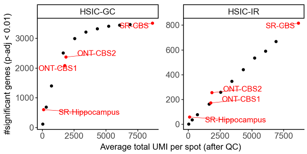
Number of significant genes versus sequencing depth in down-sampling experiments. Each black dot represents a short-read Visium coronal brain section (CBS) sample down-sampled to specific depth. ONT-CBS1 and ONT-CBS2 are two long-read SiT (Visium-ONT) CBS samples. SR-Hippocampus: Slide-seqV2 hippocampus sample with higher spatial resolution but fewer UMIs per spot.#
12. I have finished running SPLISOSM. What should I do next?
After obtaining the test results from SPLISOSM, you can perform various downstream analyses to gain further biological insights. Examples include:
Visualizing the spatial expression and usage patterns of top SVE/SVP genes.
Clustering spots or genes based on isoform usage profiles to identify spatial domains or co-regulated gene modules.
Performing Gene Ontology (GO) enrichment analysis on SVE/SVP gene lists to identify enriched biological processes.
Conducting motif enrichment analysis on the sequences of SVP genes/isoforms to identify potential regulatory elements.
Validating predicted associations between SVP genes and RNA-binding proteins (RBPs) using external data (e.g., from CLIP-seq databases like POSTAR3) or functional perturbation experiments.
Example analyses from the SPLISOSM manuscript are available in the SPLISOSM Paper GitHub Repository.