Visium HD FFPE (probe)

This notebook demonstrates a spatial exon/junction variability workflow on probe-based Visium HD data (10x Genomics):

1. Load probe-level SpatialData from Space Ranger outputs.

2. Visualize probe-level expression and within-gene ratios.

3. Run FFT-accelerated spatial variability tests with SplisosmFFT.

4. (Advanced) Check sensitivity to kernel hyperparameters and compare SplisosmFFT with SplisosmNP.

Estimated runtime: ~10 min (excluding the SplisosmNP comparison).

Preliminary notes

Visium HD probe-level data from Space Ranger (raw_probe_bc_matrix.h5, see 10x official docs) are sparse and may contain technical noise. We load data into a SpatialData object and apply quality control: barcode filtering (filtered_counts_file=True) removes barcodes dominated by ambient RNA, and probe filtering (min_counts, min_bin_pct) retains well-supported probes.

Due to Space Ranger output data structure changes, if you encounter issues, please re-run the Space Ranger (>=v4.0) count pipeline. See 10x documentation for guidance.

SplisosmFFT and SplisosmNP both implement the same HSIC-based spatial variability test but with different approaches: FFT uses full-rank kernels on regular grids (faster for large datasets); NP uses low-rank kernel approximation, compatible with irregular geometries such as cell-segmented data. For data on a regular grid — like Visium HD bins — SplisosmFFT is recommended. See the API documentation and associated preprint for technical details.

Imports

from __future__ import annotations

from itertools import combinations
from pathlib import Path
import warnings

import annsel as an
import numpy as np
import pandas as pd
import matplotlib.pyplot as plt
from scipy.stats import spearmanr

import spatialdata as sd
import spatialdata_plot
from spatialdata import rasterize_bins

from splisosm import SplisosmFFT, SplisosmNP
from splisosm.utils import counts_to_ratios
from splisosm.io import load_visiumhd_probe

/Users/jysumac/miniforge3/envs/splisosm_test/lib/python3.12/site-packages/tqdm/auto.py:21: TqdmWarning: IProgress not found. Please update jupyter and ipywidgets. See https://ipywidgets.readthedocs.io/en/stable/user_install.html
  from .autonotebook import tqdm as notebook_tqdm

warnings.filterwarnings("ignore", category=FutureWarning)
plt.rcParams["figure.dpi"] = 120
plt.rcParams["figure.figsize"] = (6, 4)

Configure paths and core parameters

# Required: Space Ranger `outs` directory for Visium HD
# visium_hd_outs = Path("/path/to/visium_hd_ffpe/outs")
visium_hd_outs = Path("/Users/jysumac/Projects/SPLISOSM_paper/data/visiumhd_ffpe_mouse_cbs/")

# Optional cache path for faster reruns
sdata_zarr = visium_hd_outs / "sdata_probe.filtered.zarr"

# Spatial resolutions (µm) to materialize in SpatialData
bin_sizes = [2, 8, 16]

# Dataset and table identifiers (16µm binning used throughout)
dataset_id = "Visium_HD_Mouse_Brain"
test_table = "square_016um"
test_bins_element = f"{dataset_id}_square_016um"

# Probe annotation column names
group_iso_by = "gene_ids"
candidate_gene_name_cols = ["gene_name", "gene_symbol", "gene_names"]

# Probe QC filters
min_counts = 10
min_bin_pct = 0.01

Load probe-level SpatialData

We use a Visium HD mouse brain FFPE dataset from 10x Genomics (Visium Mouse Transcriptome Probe Set v2.1). The probe-level SpatialData is built directly from Space Ranger outputs with load_visiumhd_probe, which wraps spatialdata-io.visium_hd.

%%time
if sdata_zarr.exists():
    print("Loading cached SpatialData...")
    sdata = sd.read_zarr(sdata_zarr)
else:
    print("Building probe-level SpatialData from Space Ranger outputs...")
    sdata = load_visiumhd_probe(
        path=visium_hd_outs,
        bin_sizes=bin_sizes,
        filtered_counts_file=True,
        load_all_images=False,
        var_names_make_unique=True,
        counts_layer_name="counts",
    )
    # Optional: cache for future runs
    # sdata.write(sdata_zarr)

sdata

Building probe-level SpatialData from Space Ranger outputs...

/Users/jysumac/miniforge3/envs/splisosm_test/lib/python3.12/site-packages/anndata/_core/anndata.py:1794: UserWarning: Variable names are not unique. To make them unique, call `.var_names_make_unique`.
/Users/jysumac/miniforge3/envs/splisosm_test/lib/python3.12/site-packages/anndata/_core/anndata.py:1794: UserWarning: Variable names are not unique. To make them unique, call `.var_names_make_unique`.
/Users/jysumac/miniforge3/envs/splisosm_test/lib/python3.12/site-packages/anndata/_core/anndata.py:1794: UserWarning: Variable names are not unique. To make them unique, call `.var_names_make_unique`.

Found segmentation data. Incorporating cell_segmentations.

/Users/jysumac/miniforge3/envs/splisosm_test/lib/python3.12/site-packages/anndata/_core/anndata.py:1794: UserWarning: Variable names are not unique. To make them unique, call `.var_names_make_unique`.
/Users/jysumac/miniforge3/envs/splisosm_test/lib/python3.12/site-packages/anndata/_core/anndata.py:1794: UserWarning: Variable names are not unique. To make them unique, call `.var_names_make_unique`.

CPU times: user 1min 48s, sys: 14.1 s, total: 2min 2s
Wall time: 2min 8s

SpatialData object
├── Images
│     ├── 'Visium_HD_Mouse_Brain_full_image': DataTree[cyx] (3, 23947, 18872), (3, 11973, 9436), (3, 5986, 4718), (3, 2993, 2359), (3, 1496, 1179)
│     ├── 'Visium_HD_Mouse_Brain_hires_image': DataArray[cyx] (3, 6000, 4729)
│     └── 'Visium_HD_Mouse_Brain_lowres_image': DataArray[cyx] (3, 600, 473)
├── Shapes
│     ├── 'Visium_HD_Mouse_Brain_cell_segmentations': GeoDataFrame shape: (40222, 2) (2D shapes)
│     ├── 'Visium_HD_Mouse_Brain_square_002um': GeoDataFrame shape: (6296688, 1) (2D shapes)
│     ├── 'Visium_HD_Mouse_Brain_square_008um': GeoDataFrame shape: (393543, 1) (2D shapes)
│     └── 'Visium_HD_Mouse_Brain_square_016um': GeoDataFrame shape: (98917, 1) (2D shapes)
└── Tables
      ├── 'cell_segmentations': AnnData (40222, 55538)
      ├── 'square_002um': AnnData (6296688, 55538)
      ├── 'square_008um': AnnData (393543, 55538)
      └── 'square_016um': AnnData (98917, 55538)
with coordinate systems:
    ▸ 'Visium_HD_Mouse_Brain', with elements:
        Visium_HD_Mouse_Brain_full_image (Images), Visium_HD_Mouse_Brain_hires_image (Images), Visium_HD_Mouse_Brain_lowres_image (Images), Visium_HD_Mouse_Brain_cell_segmentations (Shapes), Visium_HD_Mouse_Brain_square_002um (Shapes), Visium_HD_Mouse_Brain_square_008um (Shapes), Visium_HD_Mouse_Brain_square_016um (Shapes)
    ▸ 'Visium_HD_Mouse_Brain_downscaled_hires', with elements:
        Visium_HD_Mouse_Brain_hires_image (Images), Visium_HD_Mouse_Brain_cell_segmentations (Shapes), Visium_HD_Mouse_Brain_square_002um (Shapes), Visium_HD_Mouse_Brain_square_008um (Shapes), Visium_HD_Mouse_Brain_square_016um (Shapes)
    ▸ 'Visium_HD_Mouse_Brain_downscaled_lowres', with elements:
        Visium_HD_Mouse_Brain_lowres_image (Images), Visium_HD_Mouse_Brain_cell_segmentations (Shapes), Visium_HD_Mouse_Brain_square_002um (Shapes), Visium_HD_Mouse_Brain_square_008um (Shapes), Visium_HD_Mouse_Brain_square_016um (Shapes)

SPLISOSM can be run at any spatial resolution, but data become sparser at finer scales.

def summarize_table(adata):
    X = adata.layers["counts"] if "counts" in adata.layers else adata.X
    if hasattr(X, "nnz"):
        nnz = int(X.nnz)
        total = int(X.shape[0] * X.shape[1])
        density = nnz / total if total else np.nan
    else:
        arr = np.asarray(X)
        nnz = int(np.count_nonzero(arr))
        total = int(arr.size)
        density = nnz / total if total else np.nan
    return {
        "n_probes": int(adata.n_vars),
        "n_bins": int(adata.n_obs),
        "count_mtx_density": density,
    }

rows = []
for key in sorted(sdata.tables.keys()):
    if key.startswith("square_"):
        rows.append({"table": key, **summarize_table(sdata.tables[key])})

table_summary = pd.DataFrame(rows).sort_values("table")
table_summary

	table	n_probes	n_bins	count_mtx_density
0	square_002um	55538	6296688	0.000253
1	square_008um	55538	393543	0.003819
2	square_016um	55538	98917	0.013923

To balance sparsity and computation, we recommend 16µm or 8µm bins for initial analysis. Resolution comparison is shown at the end of this notebook.

# Optional: inspect available coordinate systems and image/shape keys
print("Tables:", sorted(sdata.tables.keys()))
print("Images:", sorted(getattr(sdata, "images", {}).keys()))
print("Shapes:", sorted(getattr(sdata, "shapes", {}).keys()))

# Quick guardrails before model setup
if test_table not in sdata.tables:
    raise ValueError(f"{test_table} is not available. Choose from: {sorted(sdata.tables.keys())}")

adata_test = sdata.tables[test_table]
if group_iso_by not in adata_test.var.columns:
    raise ValueError(f"{group_iso_by} not found in {test_table}.var columns")

gene_name_col = None
for col in candidate_gene_name_cols:
    if col in adata_test.var.columns:
        gene_name_col = col
        break

print(f"Using table={test_table}, bins={test_bins_element}")
print(f"Grouping column={group_iso_by}, display names={gene_name_col}")

Tables: ['cell_segmentations', 'square_002um', 'square_008um', 'square_016um']
Images: ['Visium_HD_Mouse_Brain_full_image', 'Visium_HD_Mouse_Brain_hires_image', 'Visium_HD_Mouse_Brain_lowres_image']
Shapes: ['Visium_HD_Mouse_Brain_cell_segmentations', 'Visium_HD_Mouse_Brain_square_002um', 'Visium_HD_Mouse_Brain_square_008um', 'Visium_HD_Mouse_Brain_square_016um']
Using table=square_016um, bins=Visium_HD_Mouse_Brain_square_016um
Grouping column=gene_ids, display names=gene_name

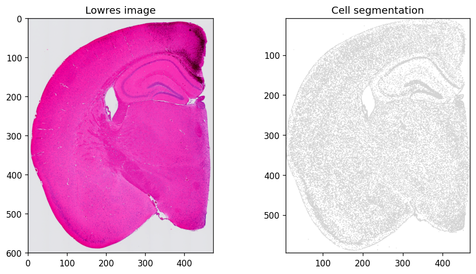
Use spatialdata-plot to visualize tissue morphology:

%%time
axes = plt.subplots(1, 2, figsize=(10, 5))[1].flatten()
sdata.pl.render_images(f"{dataset_id}_lowres_image").pl.show(
    coordinate_systems=f"{dataset_id}_downscaled_lowres",
    ax=axes[0], title="Lowres image"
)
sdata.pl.render_shapes(f"{dataset_id}_cell_segmentations").pl.show(
    coordinate_systems=f"{dataset_id}_downscaled_lowres",
    ax=axes[1], title="Cell segmentation"
)

Clipping input data to the valid range for imshow with RGB data ([0..1] for floats or [0..255] for integers). Got range [-0.5106383..1.0].

INFO     Using 'datashader' backend with 'None' as reduction method to speed up plotting. Depending on the         
         reduction method, the value range of the plot might change. Set method to 'matplotlib' to disable this    
         behaviour.                                                                                                
CPU times: user 3.58 s, sys: 258 ms, total: 3.84 s
Wall time: 4.07 s

To visualize probe expression as an image, rasterize the spatial bins first:

%%time
for bin_size in ["016", "008", "002"]:
    # rasterize_bins() requires a compressed sparse column (csc) matrix
    sdata.tables[f"square_{bin_size}um"].X = sdata.tables[f"square_{bin_size}um"].X.tocsc()
    rasterized = rasterize_bins(
        sdata,
        f"{dataset_id}_square_{bin_size}um",
        f"square_{bin_size}um",
        "array_col",
        "array_row",
    )
    sdata[f"rasterized_{bin_size}um"] = rasterized

CPU times: user 7.67 s, sys: 1.73 s, total: 9.4 s
Wall time: 10.2 s

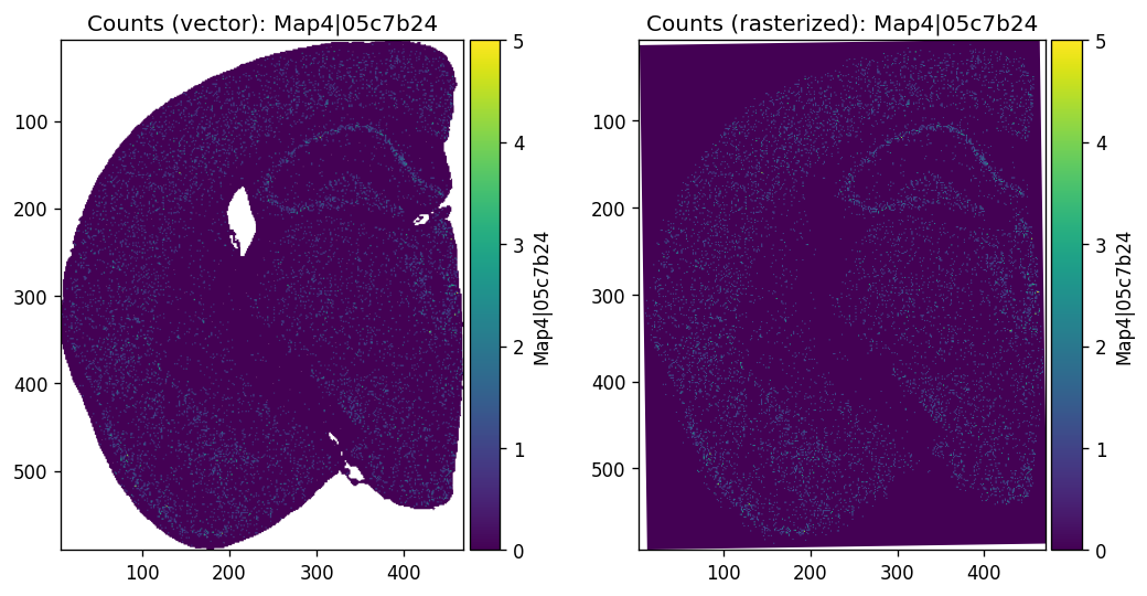
Then visualize a probe’s global expression at 16µm resolution:

%%time
probe_name = "Map4|05c7b24"
axes = plt.subplots(1, 2, figsize=(10, 5))[1].flatten()
sdata.pl.render_shapes(f"{dataset_id}_square_016um", color=probe_name).pl.show(
    coordinate_systems=f"{dataset_id}_downscaled_lowres",
    ax=axes[0], title=f"Counts (vector): {probe_name}"
)
sdata.pl.render_images(f"rasterized_016um", channel=probe_name).pl.show(
    coordinate_systems=f"{dataset_id}_downscaled_lowres",
    ax=axes[1], title=f"Counts (rasterized): {probe_name}"
)
plt.subplots_adjust(wspace=0.3)
plt.show()

INFO     Using 'datashader' backend with 'None' as reduction method to speed up plotting. Depending on the         
         reduction method, the value range of the plot might change. Set method to 'matplotlib' to disable this    
         behaviour.                                                                                                
INFO     Using the datashader reduction "mean". "max" will give an output very close to the matplotlib result.     

CPU times: user 11.1 s, sys: 4.38 s, total: 15.5 s
Wall time: 18.6 s

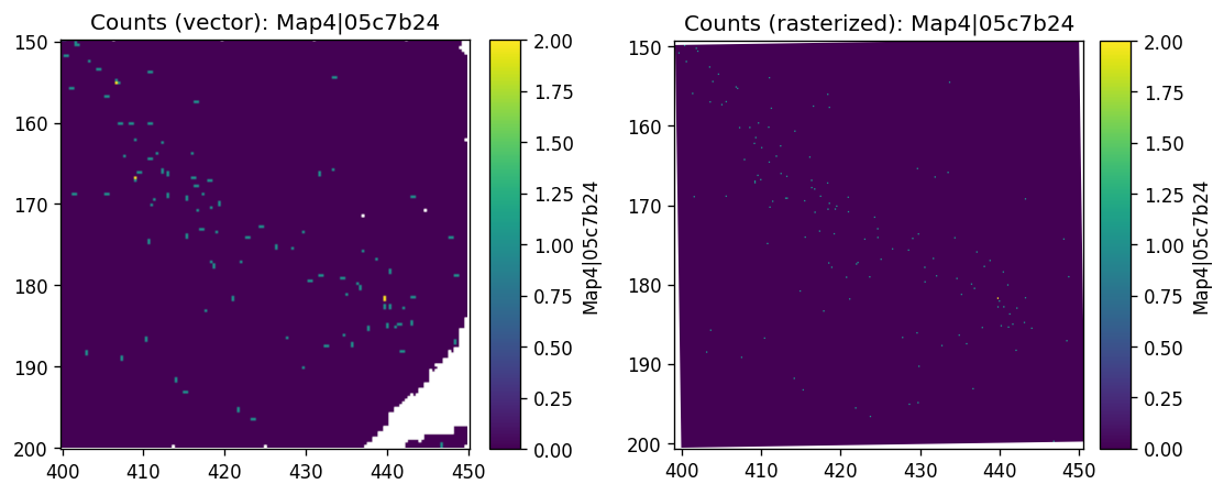
Or a zoomed-in view at a subregion (2µm resolution):

%%time
sdata_small = sdata.query.bounding_box(
    min_coordinate=[400, 150],
    max_coordinate=[450, 200],
    axes=("x", "y"),
    target_coordinate_system=f"{dataset_id}_downscaled_lowres",
)

axes = plt.subplots(1, 2, figsize=(10, 5))[1].flatten()
sdata_small.pl.render_shapes(f"{dataset_id}_square_002um", color=probe_name).pl.show(
    coordinate_systems=f"{dataset_id}_downscaled_lowres",
    ax=axes[0], title=f"Counts (vector): {probe_name}"
)
sdata_small.pl.render_images(f"rasterized_002um", channel=probe_name).pl.show(
    coordinate_systems=f"{dataset_id}_downscaled_lowres",
    ax=axes[1], title=f"Counts (rasterized): {probe_name}"
)
plt.subplots_adjust(wspace=0.5)
plt.show()

INFO     Using 'datashader' backend with 'None' as reduction method to speed up plotting. Depending on the         
         reduction method, the value range of the plot might change. Set method to 'matplotlib' to disable this    
         behaviour.                                                                                                
INFO     Using the datashader reduction "mean". "max" will give an output very close to the matplotlib result.     

CPU times: user 6.87 s, sys: 2.35 s, total: 9.22 s
Wall time: 14.4 s

Spatial variability testing with SplisosmFFT

To detect probe usage variation within a given gene, we run spatial variability test using hsic-ir.

Data filtering and model setup

Probe filtering criteria:

• min_counts: minimum total UMI count across all bins.

• min_bin_pct: minimum fraction of bins in which a probe must be detected.

• Genes with fewer than two passing probes are automatically excluded.

model = SplisosmFFT(neighbor_degree=1, rho=0.99)
model.setup_data(
    sdata=sdata,
    bins=test_bins_element,
    table_name=test_table,
    col_key="array_col",
    row_key="array_row",
    layer="counts",
    group_iso_by=group_iso_by,
    gene_names=gene_name_col, # 'gene_name'
    min_counts=min_counts,
    min_bin_pct=min_bin_pct,
)
print(model)

=== FFT SPLISOSM model for spatial isoform testings
- Number of genes: 6224
- Number of observed spots: 98917
- Number of raster cells: 124344
- Average number of isoforms per gene: 2.7485539845758353
=== Test results
- Spatial variability test: NA
- Differential usage test: NA

Extract gene-level summary statistics:

%%time
gene_meta = model.extract_feature_summary(level='gene')
gene_meta.sort_values('perplexity', ascending=False).head(5)

Genes: 100%|██████████| 6224/6224 [00:10<00:00, 605.81it/s]

CPU times: user 9.81 s, sys: 675 ms, total: 10.5 s
Wall time: 11.2 s

	n_isos	perplexity	pct_bin_on	count_avg	count_std
gene
Lrp1b	9	6.876322	0.204121	0.297128	0.723107
Shank3	6	5.873075	0.228313	0.283612	0.582347
Dusp3	6	5.868889	0.145162	0.171143	0.451044
Auts2	6	5.863693	0.142402	0.176431	0.486012
Mrtfb	6	5.777855	0.091410	0.104815	0.354134

Probe-level summary is also available:

probe_meta = model.extract_feature_summary(level='isoform')
probe_meta.sort_values('gene_name', ascending=False).head(5)

	gene_ids	probe_ids	feature_types	filtered_probes	gene_name	genome	probe_region	pct_bin_on	count_total	count_avg	count_std	ratio_total	ratio_avg	ratio_std
Zzz3|e6db6c7	ENSMUSG00000039068	ENSMUSG00000039068|Zzz3|e6db6c7	Gene Expression	True	Zzz3	GRCm39	unspliced	0.010160	1021.0	0.010322	0.102658	0.313671	0.314407	0.460947
Zzz3|78e9dcb	ENSMUSG00000039068	ENSMUSG00000039068|Zzz3|78e9dcb	Gene Expression	True	Zzz3	GRCm39	unspliced	0.011302	1141.0	0.011535	0.108935	0.350538	0.350133	0.473619
Zzz3|208a79a	ENSMUSG00000039068	ENSMUSG00000039068|Zzz3|208a79a	Gene Expression	True	Zzz3	GRCm39	unspliced	0.010787	1093.0	0.011050	0.107114	0.335791	0.335460	0.469648
Zyx|7e650fc	ENSMUSG00000029860	ENSMUSG00000029860|Zyx|7e650fc	Gene Expression	True	Zyx	GRCm39	unspliced	0.013183	1339.0	0.013537	0.118664	0.504902	0.507246	0.495824
Zyx|680c694	ENSMUSG00000029860	ENSMUSG00000029860|Zyx|680c694	Gene Expression	True	Zyx	GRCm39	spliced	0.012819	1313.0	0.013274	0.118524	0.495098	0.492754	0.495824

Running spatial variability test

%%time

model.test_spatial_variability(
    method="hsic-ir",
    ratio_transformation="none",
    n_jobs=-1,
    print_progress=True,
)
sv_res_16um = model.get_formatted_test_results("sv").sort_values("pvalue_adj")

SV (hsic-ir): 100%|██████████| 6224/6224 [03:16<00:00, 31.65it/s]

CPU times: user 5min 14s, sys: 42.2 s, total: 5min 57s
Wall time: 3min 16s

Top genes, sorted by adjusted p-value:

sig_001 = int((sv_res_16um["pvalue_adj"] < 0.01).sum())
print(
    "Spatially variably processed genes (FDR < 0.01, 16um): "
    f"{sig_001} out of {sv_res_16um.shape[0]} total genes"
)
sv_res_16um.head(5)

Spatially variably processed genes (FDR < 0.01, 16um): 192 out of 6224 total genes

	gene	statistic	pvalue	pvalue_adj
3964	Syt1	0.000003	0.000000e+00	0.000000e+00
3517	Map4	0.000005	0.000000e+00	0.000000e+00
1805	Gabbr1	0.000003	2.528068e-257	5.244899e-254
1463	Oxr1	0.000002	8.884746e-135	1.382467e-131
2276	Rabgap1l	0.000003	6.476995e-81	8.062563e-78

Merge gene-level summary back into results:

sv_res_16um.merge(
    gene_meta.reset_index()[['gene', 'n_isos', 'perplexity', 'pct_bin_on']],
    on='gene',
    how='left',
).head(5)

	gene	statistic	pvalue	pvalue_adj	n_isos	perplexity	pct_bin_on
0	Syt1	0.000003	0.000000e+00	0.000000e+00	3	2.628424	0.387153
1	Map4	0.000005	0.000000e+00	0.000000e+00	6	5.579242	0.347968
2	Gabbr1	0.000003	2.528068e-257	5.244899e-254	6	5.344769	0.283450
3	Oxr1	0.000002	8.884746e-135	1.382467e-131	5	4.394658	0.203888
4	Rabgap1l	0.000003	6.476995e-81	8.062563e-78	6	5.325925	0.242779

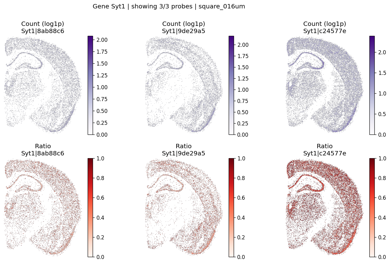
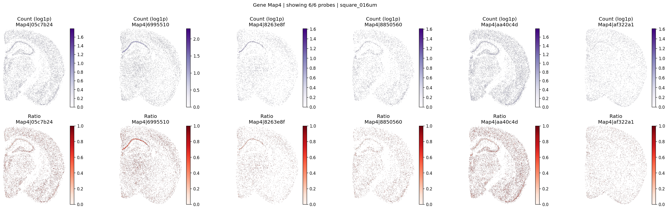
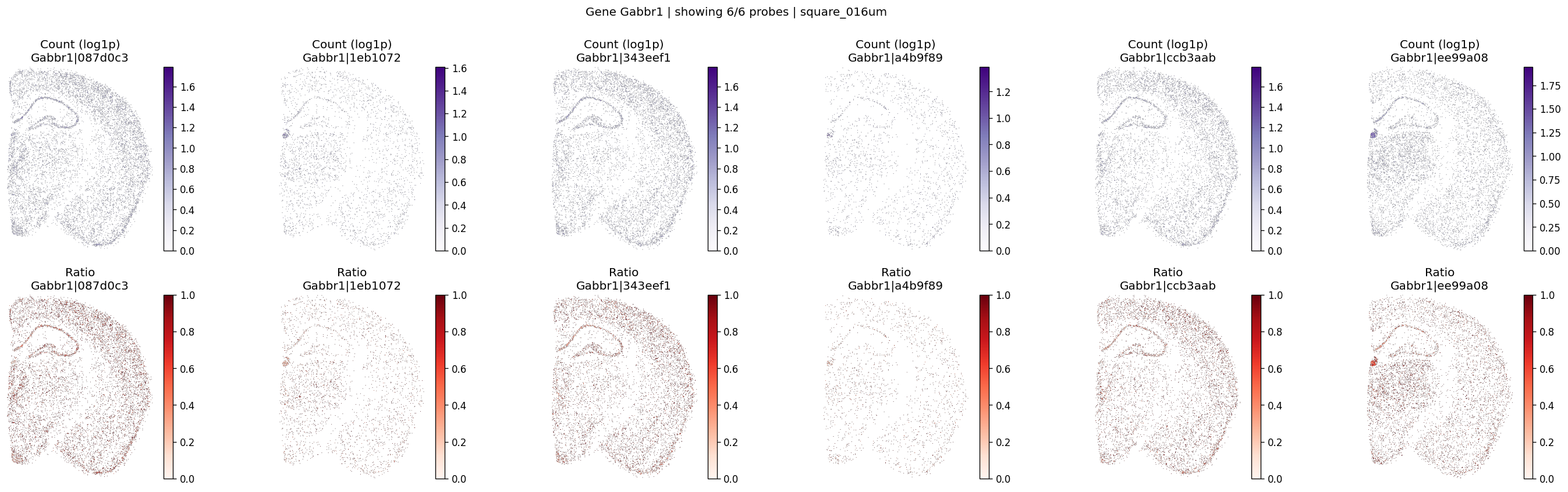
Visualize significant events

The helper below renders per-probe log1p counts and within-gene ratios on the testing grid.

def ensure_rasterized(sdata, bin_table: str, bin_element: str, layer: str = "counts"):
    raster_key = f"rasterized_{bin_table}_{layer}"
    if raster_key in sdata.images:
        return raster_key

    adata = sdata.tables[bin_table]
    adata.X = adata.layers[layer]
    if hasattr(adata.X, "tocsc") and getattr(adata.X, "format", None) != "csc":
        adata.X = adata.X.tocsc()

    sdata[raster_key] = rasterize_bins(
        sdata,
        bins=bin_element,
        table_name=bin_table,
        col_key="array_col",
        row_key="array_row",
    )
    return raster_key

The plotting function checks probe availability, lazily rasterizes data on demand, computes log1p counts and within-gene ratios, and optionally masks zero values.

def plot_gene_probe_maps(
    sdata,
    bin_table: str,
    bin_element: str,
    gene_id: str,
    probe_meta: pd.DataFrame | None = None,
    group_col: str = "gene_ids",
    max_probes: int = 4,
    hide_zero_count: bool = True,
    hide_zero_ratio: bool = True,
):
    adata = sdata.tables[bin_table]
    if probe_meta is None:
        probe_meta = adata.var.copy()

    if group_col not in probe_meta.columns:
        raise ValueError(f"'{group_col}' not found in probe_meta columns")

    probe_names = probe_meta.index[
        probe_meta[group_col].astype(str) == str(gene_id)
    ].tolist()
    if len(probe_names) == 0:
        raise ValueError(f"No probes found for gene id '{gene_id}'")
    if any(probe not in adata.var_names for probe in probe_names):
        raise ValueError(f"Some probes not found in {bin_table}.var_names")
    n_probes = len(probe_names)
    n_shown = min(n_probes, max_probes)
    probe_names = probe_names[:n_shown]

    raster_key = ensure_rasterized(sdata, bin_table=bin_table, bin_element=bin_element)
    data = sdata[raster_key].sel(c=probe_names).values
    counts_cube = np.moveaxis(np.asarray(data, dtype=float), 0, -1)

    counts_flat = counts_cube.reshape(-1, counts_cube.shape[-1])
    ratios_flat = counts_to_ratios(counts_flat, transformation="none", nan_filling="none")
    ratios_cube = ratios_flat.numpy().reshape(counts_cube.shape)

    n_probe = counts_cube.shape[-1]
    fig, axes = plt.subplots(2, n_probe, figsize=(4 * n_probe, 7), squeeze=False)

    for i, probe in enumerate(probe_names):
        c = counts_cube[:, :, i]
        r = ratios_cube[:, :, i]
        if hide_zero_count:
            c = np.where(c == 0, np.nan, c)
        if hide_zero_ratio:
            r = np.where(r == 0, np.nan, r)

        im0 = axes[0, i].imshow(np.log1p(c), cmap="Purples", vmin=0.0)
        axes[0, i].set_title(f"Count (log1p)\n{probe}")
        axes[0, i].axis("off")
        fig.colorbar(im0, ax=axes[0, i], fraction=0.046, pad=0.04)

        vmax = np.nanpercentile(ratios_cube, 99) if np.isfinite(ratios_cube).any() else 1.0
        im1 = axes[1, i].imshow(r, cmap="Reds", vmin=0.0, vmax=vmax)
        axes[1, i].set_title(f"Ratio\n{probe}")
        axes[1, i].axis("off")
        fig.colorbar(im1, ax=axes[1, i], fraction=0.046, pad=0.04)

    fig.suptitle(f"Gene {gene_id} | showing {n_shown}/{n_probes} probes | {bin_table}", y=1)
    fig.tight_layout()
    plt.show()

top_genes = sv_res_16um.head(10)["gene"].astype(str).tolist()
top_genes[:5]

['Syt1', 'Map4', 'Gabbr1', 'Oxr1', 'Rabgap1l']

for gene_id in top_genes[:3]:
    plot_gene_probe_maps(
        sdata=sdata,
        bin_table=test_table,
        bin_element=test_bins_element,
        gene_id=gene_id,
        group_col='gene_name',
        max_probes=6,
        probe_meta=probe_meta,
        hide_zero_ratio=True,
    )

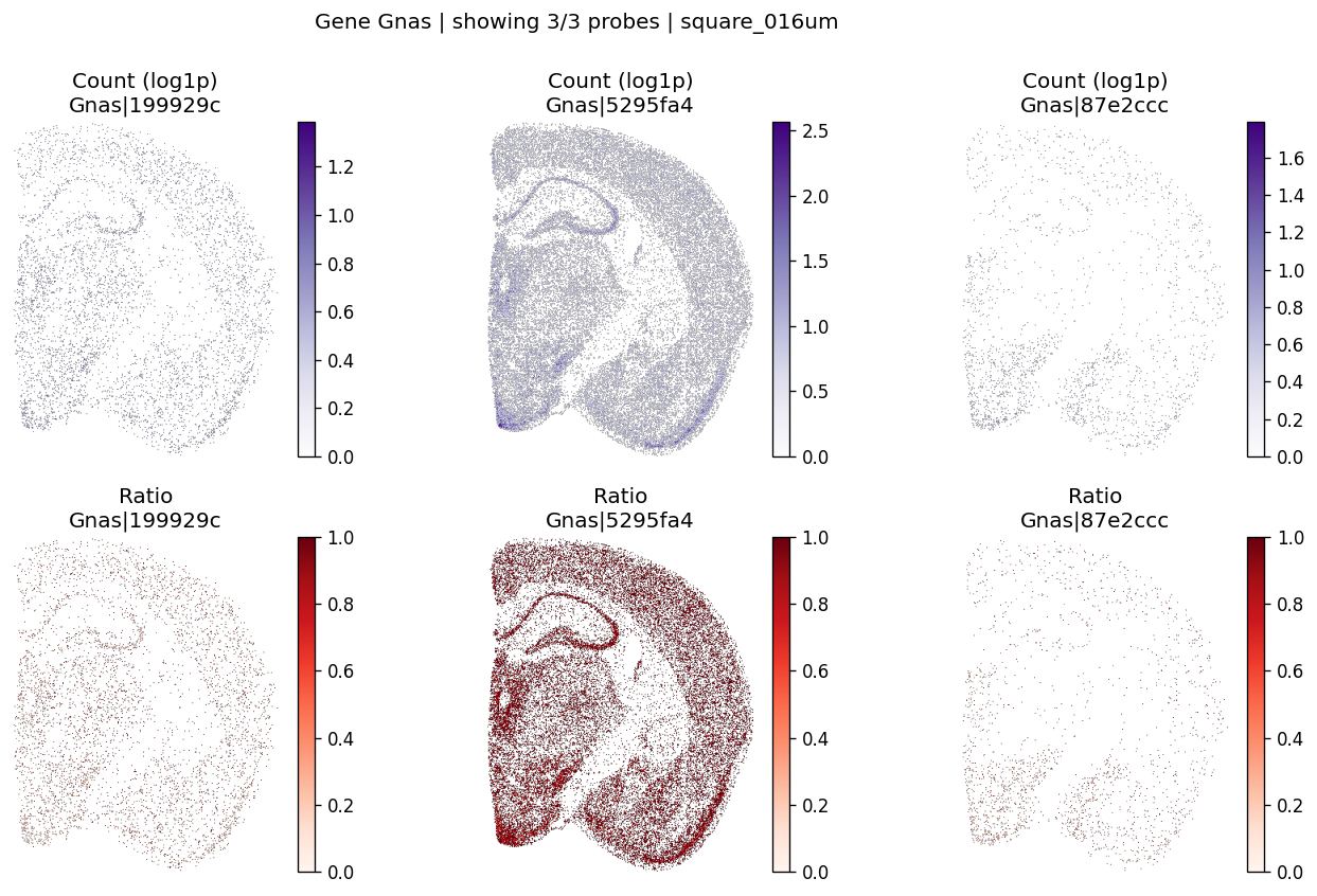
%%time
# Example: inspect a specific gene manually
plot_gene_probe_maps(
    sdata, test_table, test_bins_element, 
    gene_id="Gnas", 
    group_col='gene_name', 
    probe_meta=probe_meta
)

CPU times: user 370 ms, sys: 24.8 ms, total: 395 ms
Wall time: 525 ms

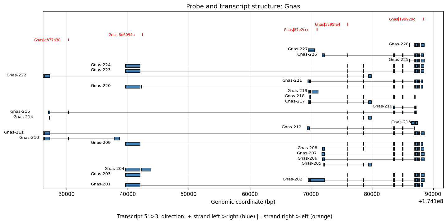
To see the spatially variable transcript regions, we can visualize the 10x reference probe sets along with a matched transcript reference. The following files need to be downloaded and provided as input:

• Visium_Mouse_Transcriptome_Probe_Set_v2.1.0_GRCm39-2024-A.bed from 10x Genomics

• gencode.vM33.annotation.gtf.gz from GENCODE

Show code cell source

Hide code cell source

def plot_probe_transcript_structure(
    gene_name: str,
    bed_file: str | Path,
    gtf_file: str | Path,
    figsize: tuple[float, float] = (12, 6),
):
    """Visualize probe and transcript exon structure for a given gene.

    Reads probe coordinates from a BED12 file and transcript structure from a GTF file,
    then plots them on the same genomic coordinate axis. Each probe is shown on its
    own row to avoid overlap, and transcripts are labeled by transcript_name.
    """
    import gzip

    bed_file = Path(bed_file)
    gtf_file = Path(gtf_file)

    # Read BED12 file and keep block model columns.
    bed_cols = [
        "chrom", "start", "end", "name", "score", "strand",
        "thickStart", "thickEnd", "itemRgb", "blockCount", "blockSizes", "blockStarts",
    ]
    bed_df = pd.read_csv(
        bed_file,
        sep="\t",
        header=None,
        names=bed_cols,
        usecols=list(range(12)),
    )

    # Filter probes that match gene name (probe names often include gene symbol).
    probe_mask = bed_df["name"].astype(str).str.contains(gene_name, case=False, na=False)
    probes = bed_df[probe_mask].copy()

    if probes.empty:
        warnings.warn(f"No probes found for gene '{gene_name}' in {bed_file}")

    # Extract shorter probe labels for common formats.
    def shorten_probe_id(full_name: str) -> str:
        text = str(full_name)
        if "|" in text:
            parts = text.split("|")
            if len(parts) >= 2:
                return "|".join(parts[1:])
        return text

    probes["probe_id"] = probes["name"].apply(shorten_probe_id)

    # Convert BED12 blocks to absolute genomic coordinates per probe.
    def parse_blocks(row: pd.Series) -> list[tuple[int, int]]:
        starts = [int(x) for x in str(row["blockStarts"]).strip(",").split(",") if x != ""]
        sizes = [int(x) for x in str(row["blockSizes"]).strip(",").split(",") if x != ""]
        n = min(int(row["blockCount"]), len(starts), len(sizes))
        blocks = []
        for i in range(n):
            block_start = int(row["start"]) + starts[i]
            block_end = block_start + sizes[i]
            blocks.append((block_start, block_end))
        return blocks

    if not probes.empty:
        probes["blocks"] = probes.apply(parse_blocks, axis=1)

    # Read GTF and filter transcripts by gene name
    if str(gtf_file).endswith(".gz"):
        gtf_opener = lambda f: gzip.open(f, "rt")
    else:
        gtf_opener = open

    transcripts_by_id = {}
    with gtf_opener(gtf_file) as f:
        for line in f:
            if line.startswith("#"):
                continue
            fields = line.rstrip("\n").split("\t")
            if len(fields) < 9:
                continue
            ftype, start, end = fields[2], int(fields[3]), int(fields[4])
            attrs = {}
            for attr in fields[8].split("; "):
                if " " in attr:
                    k, v = attr.split(" ", 1)
                    attrs[k] = v.strip('"')

            # Match gene by gene_name or gene_id
            if attrs.get("gene_name", "").lower() != gene_name.lower() and \
               attrs.get("gene_id", "").lower() != gene_name.lower():
                continue

            tx_id = attrs.get("transcript_id", "unknown")
            if tx_id not in transcripts_by_id:
                tx_name = attrs.get("transcript_name", tx_id)
                transcripts_by_id[tx_id] = {
                    "chrom": fields[0],
                    "strand": fields[6],
                    "tx_name": tx_name,
                    "exons": [],
                }

            if ftype == "exon":
                transcripts_by_id[tx_id]["exons"].append((start, end))

    # Create plot
    fig, ax = plt.subplots(figsize=figsize)

    # Plot transcripts first
    y_pos = 0
    x_mins = []
    x_maxs = []

    # Strand color coding for cleaner direction cues.
    strand_colors = {
        "+": "steelblue",
        "-": "darkorange",
    }

    if transcripts_by_id:
        for tx_id, tx_info in sorted(transcripts_by_id.items()):
            exons = sorted(tx_info["exons"])
            if not exons:
                continue

            # Draw introns (thin line)
            min_coord = min(e[0] for e in exons)
            max_coord = max(e[1] for e in exons)
            x_mins.append(min_coord)
            x_maxs.append(max_coord)
            ax.plot([min_coord, max_coord], [y_pos, y_pos], "k-", linewidth=0.5, alpha=0.5)

            # Draw exons (thick boxes), color by strand
            strand = str(tx_info.get("strand", "."))
            tx_color = strand_colors.get(strand, "gray")
            for start, end in exons:
                ax.barh(y_pos, end - start, left=start, height=0.6, color=tx_color, edgecolor="black")

            # Label with transcript_name
            tx_name = tx_info.get("tx_name", tx_id[:20])
            ax.text(min_coord - (max_coord - min_coord) * 0.05, y_pos, tx_name[:30], ha="right", fontsize=8)
            y_pos += 1

    # Plot probes, each on its own row, using BED12 block segments.
    probe_rows = probes.sort_values(["chrom", "start", "end"]) if not probes.empty else probes

    for idx, (_, row) in enumerate(probe_rows.iterrows()):
        probe_y = y_pos + idx
        blocks = row["blocks"] if isinstance(row["blocks"], list) and row["blocks"] else [(int(row["start"]), int(row["end"]))]
        probe_min = min(b[0] for b in blocks)
        probe_max = max(b[1] for b in blocks)
        x_mins.append(probe_min)
        x_maxs.append(probe_max)

        ax.plot([probe_min, probe_max], [probe_y, probe_y], color="firebrick", linewidth=0.7, alpha=0.6)
        for block_start, block_end in blocks:
            ax.barh(
                probe_y,
                block_end - block_start,
                left=block_start,
                height=0.45,
                color="salmon",
                edgecolor="firebrick",
            )

    x_pad = max(1.0, (max(x_maxs) - min(x_mins)) * 0.02) if x_mins and x_maxs else 1.0

    for idx, (_, row) in enumerate(probe_rows.iterrows()):
        probe_y = y_pos + idx
        blocks = row["blocks"] if isinstance(row["blocks"], list) and row["blocks"] else [(int(row["start"]), int(row["end"]))]
        probe_min = min(b[0] for b in blocks)
        ax.text(probe_min - x_pad, probe_y, row["probe_id"], ha="right", va="center", fontsize=7, color="red")

    y_pos += len(probe_rows)

    # Format axes
    ax.set_ylim(-0.5, y_pos + 0.5)
    ax.set_xlabel("Genomic coordinate (bp)")
    ax.set_ylabel("")
    ax.set_yticks([])
    ax.set_title(f"Probe and transcript structure: {gene_name}")
    ax.grid(True, axis="x", alpha=0.3)

    # Place strand direction note as a single centered row below the plot.
    direction_note = "Transcript 5'->3' direction: + strand left->right (blue) | - strand right->left (orange)"
    fig.text(0.5, 0.01, direction_note, ha="center", va="bottom", fontsize=10, color="black")

    # Reserve bottom margin for the legend row.
    fig.tight_layout(rect=(0.0, 0.05, 1.0, 1.0))
    plt.show()

%%time
plot_probe_transcript_structure(
    gene_name="Gnas",
    bed_file=visium_hd_outs / "Visium_Mouse_Transcriptome_Probe_Set_v2.1.0_GRCm39-2024-A.bed",
    gtf_file="/Users/jysumac/reference/mm39/gencode.vM33.annotation.gtf.gz",
)

CPU times: user 10.8 s, sys: 103 ms, total: 10.9 s
Wall time: 11.2 s

Advanced analyses

Hyperparameter sensitivity check

A lightweight robustness check compares p-values under nearby kernel settings (neighbor_degree, rho).

# reusable setup parameters for multiple resolutions
setup_params = {
    'sdata': sdata,
    'bins': test_bins_element,
    'table_name': test_table,
    'col_key': "array_col",
    'row_key': "array_row",
    'layer': "counts",
    'group_iso_by': group_iso_by,
    'gene_names': gene_name_col,
    'min_counts': 100,
    'min_bin_pct': 0.05,
}

Spectral analysis of kernel matrices

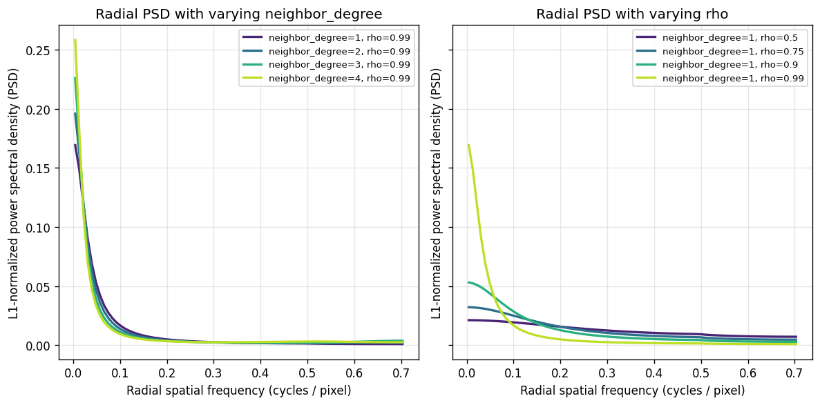
Two hyperparameters control the kernel: neighbor_degree (spatial graph connectivity; larger values capture more global structure) and rho (spectral decay; values closer to 1 concentrate energy on low-frequency patterns). The plots below show the normalized power spectral density under different settings.

%%time
def extract_l1_normalized_psd(model, bins=80):
    """Return radial PSD with L1 normalization for comparison across kernels."""
    freq_bins, psd = model.kernel.power_spectral_density_1d(bins=bins)
    # scale eigenvalues to sum-one
    denom = float(np.sum(np.abs(psd)))
    if denom <= 0.0:
        raise ValueError("Power spectral density has zero total magnitude.")
    return freq_bins, psd / denom


def plot_psd_family(configs, title, ax, bins=80):
    colors = plt.cm.viridis(np.linspace(0.1, 0.9, len(configs)))

    for cfg, color in zip(configs, colors):
        m = SplisosmFFT(**cfg)
        m.setup_data(**setup_params)
        freq_bins, psd_l1 = extract_l1_normalized_psd(m, bins=bins)
        label = ", ".join([f"{key}={value}" for key, value in cfg.items()])
        ax.plot(freq_bins, psd_l1, color=color, linewidth=2.0, label=label)

    ax.set_xlabel("Radial spatial frequency (cycles / pixel)")
    ax.set_ylabel("L1-normalized power spectral density (PSD)")
    ax.set_title(title)
    ax.grid(True, alpha=0.3)
    ax.legend(fontsize=8)


neighbor_configs = [
    {"neighbor_degree": 1, "rho": 0.99},
    {"neighbor_degree": 2, "rho": 0.99},
    {"neighbor_degree": 3, "rho": 0.99},
    {"neighbor_degree": 4, "rho": 0.99},
]

rho_configs = [
    {"neighbor_degree": 1, "rho": 0.50},
    {"neighbor_degree": 1, "rho": 0.75},
    {"neighbor_degree": 1, "rho": 0.90},
    {"neighbor_degree": 1, "rho": 0.99},
]

fig, axes = plt.subplots(1, 2, figsize=(10, 5), sharey=True)
plot_psd_family(
    neighbor_configs,
    title="Radial PSD with varying neighbor_degree",
    ax=axes[0],
    bins=80,
)
plot_psd_family(
    rho_configs,
    title="Radial PSD with varying rho",
    ax=axes[1],
    bins=80,
)
plt.tight_layout()
plt.show()

CPU times: user 37.6 s, sys: 3.24 s, total: 40.9 s
Wall time: 42.3 s

rho is the more effective parameter for emphasizing low-frequency spatial patterns.

Effect on spatial variability results

Compare gene rankings across hyperparameter settings:

%%time
configs = [
    {"neighbor_degree": 1, "rho": 0.99},
    {"neighbor_degree": 2, "rho": 0.99},
    {"neighbor_degree": 1, "rho": 0.90},
]

cfg_results = []
for cfg in configs:
    m = SplisosmFFT(neighbor_degree=cfg["neighbor_degree"], rho=cfg["rho"])
    m.setup_data(**setup_params)
    m.test_spatial_variability(
        method='hsic-ir',
        ratio_transformation='none',
        n_jobs=-1,
        print_progress=True,
    )
    res = m.get_formatted_test_results("sv")[["gene", "pvalue", "pvalue_adj"]].copy()
    tag = f"k{cfg['neighbor_degree']}_rho{cfg['rho']}"
    res = res.rename(columns={"pvalue": f"p_{tag}", "pvalue_adj": f"padj_{tag}"})
    cfg_results.append(res)

SV (hsic-ir): 100%|██████████| 1065/1065 [00:31<00:00, 33.97it/s]
SV (hsic-ir): 100%|██████████| 1065/1065 [00:33<00:00, 32.23it/s]
SV (hsic-ir): 100%|██████████| 1065/1065 [00:31<00:00, 34.30it/s]

CPU times: user 2min 47s, sys: 21.1 s, total: 3min 8s
Wall time: 1min 53s

merged = cfg_results[0]
for res in cfg_results[1:]:
    merged = merged.merge(res, on="gene", how="inner")

p_cols = [c for c in merged.columns if c.startswith("p_")]
print("Spearman correlation across hyperparameter settings:")
display(merged[p_cols].corr(method="spearman"))

Spearman correlation across hyperparameter settings:

	p_k1_rho0.99	p_k2_rho0.99	p_k1_rho0.9
p_k1_rho0.99	1.000000	0.992535	0.818226
p_k2_rho0.99	0.992535	1.000000	0.757116
p_k1_rho0.9	0.818226	0.757116	1.000000

pairs = list(combinations(p_cols, 2))
if pairs:
    fig, axes = plt.subplots(1, len(pairs), figsize=(3 * len(pairs), 3), squeeze=False)
    axes = axes.ravel()

    for ax, (x_col, y_col) in zip(axes, pairs):
        x = merged[x_col].to_numpy()
        y = merged[y_col].to_numpy()
        corr, pval = spearmanr(x, y)

        ax.scatter(x + 1e-100, y + 1e-100, s=8, alpha=0.5)
        ax.set_xscale("log")
        ax.set_yscale("log")
        ax.set_xlabel(x_col)
        ax.set_ylabel(y_col)
        ax.set_title(f"Spearman ρ={corr:.3f}")
        ax.grid(True, alpha=0.3)

        low = 1e-100
        high = max(np.max(x), np.max(y))
        ax.plot([low, high], [low, high], "r--", alpha=0.5, linewidth=1.5)
        ax.set_xlim(low, high)
        ax.set_ylim(low, high)

    plt.tight_layout()
    plt.show()

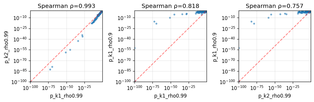
Gene rankings are more sensitive to rho than neighbor_degree. For this mouse brain dataset, most spatial patterns are low-frequency, so decreasing rho reduces statistical power.

Spatial resolution comparison

For illustration, we use the top 200 genes from the 16µm analysis as the reference set:

# np.random.seed(42)
# gene_names = sdata.tables[test_table].var['gene_name'].unique()
# gene_subset = np.random.choice(gene_names, size=200, replace=False)
gene_subset = sv_res_16um.sort_values('pvalue').head(200)['gene'].astype(str).tolist()

Run spatial variability tests across all three resolutions:

%%time
# Compare results across 2µm, 8µm, 16µm resolutions
resolutions = [
    {'bin': f'{dataset_id}_square_002um', 'table_name': 'square_002um'},
    {'bin': f'{dataset_id}_square_008um', 'table_name': 'square_008um'},
    {'bin': f'{dataset_id}_square_016um', 'table_name': 'square_016um'},
]

res_results = []
for res in resolutions:
    m = SplisosmFFT(neighbor_degree=1, rho=0.99)
    sdata_subset = sd.filter_by_table_query(
        sdata,
        table_name=res['table_name'],
        var_expr=an.col('gene_name').is_in(gene_subset),
    )
    m.setup_data(
        sdata_subset,
        bins=res['bin'],
        table_name=res['table_name'],
        col_key="array_col",
        row_key="array_row",
        layer="counts",
        group_iso_by="gene_ids",
        gene_names="gene_name",
        min_counts=10,
        min_bin_pct=0.0
    )
    m.test_spatial_variability(method='hsic-ir')
    results = m.get_formatted_test_results('sv')[['gene', 'pvalue']].copy()
    results.rename(columns={'pvalue': f"p_{res['table_name']}"}, inplace=True)
    res_results.append(results)

SV (hsic-ir): 100%|██████████| 200/200 [04:21<00:00,  1.31s/it]
SV (hsic-ir): 100%|██████████| 200/200 [00:06<00:00, 29.22it/s]
SV (hsic-ir): 100%|██████████| 200/200 [00:02<00:00, 87.99it/s]

CPU times: user 8min 9s, sys: 8min 45s, total: 16min 54s
Wall time: 5min 4s

merged = res_results[0]
for res in res_results[1:]:
    merged = merged.merge(res, on="gene", how="inner")

p_cols = [c for c in merged.columns if c.startswith("p_")]
print("Spearman correlation across spatial resolutions:")
display(merged[p_cols].corr(method="spearman"))

Spearman correlation across spatial resolutions:

	p_square_002um	p_square_008um	p_square_016um
p_square_002um	1.000000	0.611568	0.514374
p_square_008um	0.611568	1.000000	0.704984
p_square_016um	0.514374	0.704984	1.000000

pairs = list(combinations(p_cols, 2))
if pairs:
    fig, axes = plt.subplots(1, len(pairs), figsize=(3 * len(pairs), 3), squeeze=False)
    axes = axes.ravel()

    for ax, (x_col, y_col) in zip(axes, pairs):
        x = merged[x_col].to_numpy()
        y = merged[y_col].to_numpy()
        corr, pval = spearmanr(x, y)

        ax.scatter(x + 1e-150, y + 1e-150, s=8, alpha=0.5)
        ax.set_xscale("log")
        ax.set_yscale("log")
        ax.set_xlabel(x_col)
        ax.set_ylabel(y_col)
        ax.set_title(f"Spearman ρ={corr:.3f}")
        ax.grid(True, alpha=0.3)

        low = 1e-150
        high = max(np.max(x), np.max(y))
        ax.plot([low, high], [low, high], "r--", alpha=0.5, linewidth=1.5)
        ax.set_xlim(low, high)
        ax.set_ylim(low, high)

    plt.tight_layout()
    plt.show()

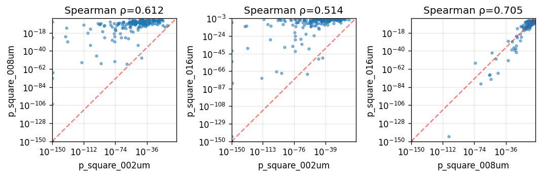
Gene rankings are broadly consistent across resolutions, especially between 16µm and 8µm. The 2µm analysis shows stronger statistical significance, likely because the kernel places more weight on low-frequency patterns at finer scales.

Method comparison: SplisosmFFT vs SplisosmNP

Compare FFT-accelerated and non-parametric spatial variability tests at 16 µm resolution.

SplisosmNP.setup_data performs low-rank kernel approximation (controlled by approx_rank). A higher rank gives more accurate approximations at increased cost. Here we use approx_rank=20 for demonstration.

%%time
# Run SplisosmNP at 16µm for direct comparison with SplisosmFFT
model_np = SplisosmNP()
model_np.setup_data(
    adata=sdata.tables[test_table],
    spatial_key='spatial', # adata.obsm key for spatial coordinates
    layer='counts',
    approx_rank=20,
    group_iso_by=group_iso_by, # 'gene_ids'
    gene_names=gene_name_col, # 'gene_name'
    min_counts=min_counts,
    min_bin_pct=min_bin_pct,
)

CPU times: user 9min 38s, sys: 6.85 s, total: 9min 45s
Wall time: 9min 28s

%%time
model_np.test_spatial_variability(
    method='hsic-ir',
    ratio_transformation='none',
    print_progress=True,
)

100%|██████████| 6224/6224 [00:30<00:00, 204.80it/s]

CPU times: user 38.5 s, sys: 2.99 s, total: 41.5 s
Wall time: 30.4 s

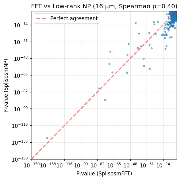
Compare p-values between SplisosmFFT and SplisosmNP:

# Extract results and merge
sv_np = model_np.get_formatted_test_results('sv')[['gene', 'pvalue']].copy()
sv_np = sv_np.rename(columns={'pvalue': 'pvalue_np'})

comparison = sv_res_16um[['gene', 'pvalue']].copy()
comparison = comparison.rename(columns={'pvalue': 'pvalue_fft'})
comparison = comparison.merge(sv_np, on='gene', how='inner')

corr, _ = spearmanr(comparison['pvalue_fft'], comparison['pvalue_np'])

print(f'Genes tested in both methods: {len(comparison)}')
print(f'== Significant in SplisosmFFT (FDR < 0.01): {(comparison["pvalue_fft"] < 0.01).sum()}')
print(f'== Significant in SplisosmNP (FDR < 0.01): {(comparison["pvalue_np"] < 0.01).sum()}')
print(f'== P-value correlation (Spearman rho): {corr:.4f}')

Genes tested in both methods: 6226
== Significant in SplisosmFFT (FDR < 0.01): 616
== Significant in SplisosmNP (FDR < 0.01): 819
== P-value correlation (Spearman rho): 0.4007

# Scatter plot comparison
fig, ax = plt.subplots(figsize=(5, 5))
x = comparison['pvalue_fft'].to_numpy()
y = comparison['pvalue_np'].to_numpy()

ax.scatter(x + 1e-150, y + 1e-150, s=8, alpha=0.5)
ax.set_xscale('log')
ax.set_yscale('log')
ax.set_xlabel('P-value (SplisosmFFT)')
ax.set_ylabel('P-value (SplisosmNP)')
ax.set_title(f'FFT vs Low-rank NP (16 µm, Spearman ρ={corr:.2f})')
ax.grid(True, alpha=0.3)

# Add diagonal reference line
lims = [1e-150, 1.0]
ax.plot(lims, lims, 'r--', alpha=0.5, label='Perfect agreement', linewidth=2)
ax.legend()
ax.set_xlim(lims)
ax.set_ylim(lims)

plt.tight_layout()
plt.show()

Summary and recommendations

Key findings:

1. Kernel spectra concentrate energy at low frequencies. Both neighbor_degree and rho shape the spectrum, but rho has the larger effect on downstream gene rankings. Kernels emphasizing low-frequency patterns tend to yield higher statistical power.

2. Spatial resolution trade-offs:

   • 16 µm: Fast and reliable — recommended for initial exploration.

   • 8 µm: High agreement with 16 µm results.

   • 2 µm: Highest resolution but slower and sparser.

3. Method equivalence: SplisosmFFT and SplisosmNP yield concordant rankings on regular grids, particularly for genes with strong spatial patterns.

Recommendations:

• Start with 16 µm binning for exploratory analysis.

• Refine with 8 µm if finer spatial detail is needed.

• Use SplisosmFFT on regular grids (Visium HD, Xenium binned data) with neighbor_degree=1, rho=0.99 as a robust default.

• Use SplisosmNP for irregular geometries (e.g., cell-segmented data).

For reproducibility

import sys
from datetime import date
import splisosm

print("Last updated:", date.today())
print("Python:", sys.version.split()[0])
print("splisosm:", getattr(splisosm, "__version__", "unknown"))

Last updated: 2026-03-17
Python: 3.12.12
splisosm: 1.0.4