Visium HD 3’ (peak)

This notebook demonstrates a spatial transcriptome 3’ end diversity (TREND) workflow on 3’ Visium HD peak-level data:

1. Load preprocessed peak-level SpatialData from a .zarr store.

2. Visualize peak-level expression and within-gene ratios.

3. Run FFT-accelerated spatial variability tests with SplisosmFFT.

4. Compare results across spatial resolutions and with SplisosmNP.

Estimated runtime: ~20 min.

Preliminary notes

3’ end sequencing data allows us to investigate variation near the 3’ end of transcripts, which we refer to as transcriptome 3’ end diversity (TREND) events. For the analysis, we first call junction-aware peaks from the BAM file using Sierra, then quantify peak-level expression in each Visium HD bin using UMI-tools. An example workflow is provided in scripts/visiumhd_3p_trend_quant.sh under the scripts directory, which generates a peak-level SpatialData object stored as a .zarr file.

SplisosmFFT and SplisosmNP both implement the same HSIC-based spatial variability test but with different approaches: FFT uses full-rank kernels on regular grids (faster for large datasets); NP uses low-rank kernel approximation, compatible with irregular geometries such as cell-segmented data. For data on a regular grid — like Visium HD bins — SplisosmFFT is recommended. See the API documentation and associated preprint for technical details.

Imports

from __future__ import annotations

from itertools import combinations
from pathlib import Path
import warnings

import annsel as an
import numpy as np
import pandas as pd
import matplotlib.pyplot as plt
from scipy.stats import spearmanr

import spatialdata as sd
import spatialdata_plot
from spatialdata import rasterize_bins

from splisosm import SplisosmFFT, SplisosmNP
from splisosm.utils import counts_to_ratios

/Users/jysumac/miniforge3/envs/splisosm_test/lib/python3.12/site-packages/tqdm/auto.py:21: TqdmWarning: IProgress not found. Please update jupyter and ipywidgets. See https://ipywidgets.readthedocs.io/en/stable/user_install.html
  from .autonotebook import tqdm as notebook_tqdm

warnings.filterwarnings("ignore", category=FutureWarning)
plt.rcParams["figure.dpi"] = 120
plt.rcParams["figure.figsize"] = (6, 4)

Configure paths and core parameters

# Path to the preprocessed peak-level SpatialData zarr
sdata_zarr = Path("/Users/jysumac/Projects/SPLISOSM_paper/data/visiumhd_3p_mouse_cbs/sdata_peak.filtered.zarr")

# Dataset and table identifiers (16um binning used throughout)
dataset_id = ""
test_table = "square_016um"
test_bins_element = f"{dataset_id}_square_016um"

# Peak annotation column names
group_iso_by = "gene_ids"
gene_name_col = "gene_ids"
candidate_gene_name_cols = ["gene_name", "gene_ids", "gene_symbol", "gene_names"]

# Peak QC filters
min_counts = 10
min_bin_pct = 0.01

Load preprocessed peak-level SpatialData

We use a Visium HD 3’ mouse brain dataset from 10x Genomics (Fresh Frozen). Here we load the preprocessed peak-level SpatialData generated from the custom quantification workflow in scripts/visiumhd_3p_trend_quant.sh. Sierra peak quantification is stored at outs/binned_outputs/square_002um/raw_probe_bc_matrix.h5.

%%time
if sdata_zarr.exists():
    print("Loading preprocessed SpatialData...")
    sdata = sd.read_zarr(sdata_zarr)
else:
    print("Building peak-level SpatialData from quantification outputs...")
    from splisosm.io import load_visiumhd_peak
    sdata = load_visiumhd_peak(
        path='path/to/outs',
        bin_sizes=bin_sizes,
        filtered_counts_file=True,
        load_all_images=False,
        var_names_make_unique=True,
        counts_layer_name="counts",
    )
    # Optional: cache for future runs
    # sdata.write(sdata_zarr)

sdata

Loading preprocessed SpatialData...
CPU times: user 11 s, sys: 3.26 s, total: 14.3 s
Wall time: 11.1 s

SpatialData object, with associated Zarr store: /Users/jysumac/Projects/SPLISOSM_paper/data/visiumhd_3p_mouse_cbs/sdata_peak.filtered.zarr
├── Images
│     ├── '_hires_image': DataArray[cyx] (3, 5492, 6000)
│     └── '_lowres_image': DataArray[cyx] (3, 549, 600)
├── Shapes
│     ├── '_cell_segmentations': GeoDataFrame shape: (84031, 2) (2D shapes)
│     ├── '_square_002um': GeoDataFrame shape: (5998466, 1) (2D shapes)
│     ├── '_square_008um': GeoDataFrame shape: (376419, 1) (2D shapes)
│     └── '_square_016um': GeoDataFrame shape: (94592, 1) (2D shapes)
└── Tables
      ├── 'cell_segmentations': AnnData (84031, 19575)
      ├── 'square_002um': AnnData (5998466, 19575)
      ├── 'square_008um': AnnData (376419, 19575)
      └── 'square_016um': AnnData (94592, 19575)
with coordinate systems:
    ▸ '', with elements:
        _hires_image (Images), _lowres_image (Images), _cell_segmentations (Shapes), _square_002um (Shapes), _square_008um (Shapes), _square_016um (Shapes)
    ▸ '_downscaled_hires', with elements:
        _hires_image (Images), _cell_segmentations (Shapes), _square_002um (Shapes), _square_008um (Shapes), _square_016um (Shapes)
    ▸ '_downscaled_lowres', with elements:
        _lowres_image (Images), _cell_segmentations (Shapes), _square_002um (Shapes), _square_008um (Shapes), _square_016um (Shapes)

SPLISOSM can be run at any spatial resolution, but data become sparser at finer scales.

def summarize_table(adata):
    X = adata.layers["counts"] if "counts" in adata.layers else adata.X
    if hasattr(X, "nnz"):
        nnz = int(X.nnz)
        total = int(X.shape[0] * X.shape[1])
        density = nnz / total if total else np.nan
    else:
        arr = np.asarray(X)
        nnz = int(np.count_nonzero(arr))
        total = int(arr.size)
        density = nnz / total if total else np.nan
    return {
        "n_peaks": int(adata.n_vars),
        "n_bins": int(adata.n_obs),
        "count_mtx_density": density,
    }

rows = []
for key in sorted(sdata.tables.keys()):
    if key.startswith("square_"):
        rows.append({"table": key, **summarize_table(sdata.tables[key])})

table_summary = pd.DataFrame(rows).sort_values("table")
table_summary

	table	n_peaks	n_bins	count_mtx_density
0	square_002um	19575	5998466	0.000437
1	square_008um	19575	376419	0.006380
2	square_016um	19575	94592	0.022677

To balance sparsity and computation, we recommend 16µm or 8µm bins for initial analysis. Resolution comparison is shown at the end of this notebook.

# Optional: inspect available coordinate systems and image/shape keys
print("Tables:", sorted(sdata.tables.keys()))
print("Images:", sorted(getattr(sdata, "images", {}).keys()))
print("Shapes:", sorted(getattr(sdata, "shapes", {}).keys()))

# Quick guardrails before model setup
if test_table not in sdata.tables:
    raise ValueError(f"{test_table} is not available. Choose from: {sorted(sdata.tables.keys())}")

adata_test = sdata.tables[test_table]
if group_iso_by not in adata_test.var.columns:
    raise ValueError(f"{group_iso_by} not found in {test_table}.var columns")

if gene_name_col not in adata_test.var.columns:
    for col in candidate_gene_name_cols:
        if col in adata_test.var.columns:
            gene_name_col = col
            break

print(f"Using table={test_table}, bins={test_bins_element}")
print(f"Grouping column={group_iso_by}, display names={gene_name_col}")

Tables: ['cell_segmentations', 'square_002um', 'square_008um', 'square_016um']
Images: ['_hires_image', '_lowres_image']
Shapes: ['_cell_segmentations', '_square_002um', '_square_008um', '_square_016um']
Using table=square_016um, bins=_square_016um
Grouping column=gene_ids, display names=gene_ids

Features in this dataset are peaks (single-exon or across junctions) called by Sierra’s FindPeaks function, and annotated by whether they overlap with coding regions (CDS), UTRs (UTR3 and UTR5), or introns of some isoforms (intron) using AnnotatePeaksFromGTF(annotation_correction=FALSE).

sdata.tables[test_table].var.head(5)

	gene_ids	probe_ids	feature_types	CDS	Junctions	UTR3	UTR5	end	exon	genome	intron	seqnames	start	strand	width
0610009B22Rik:chr11:51576213-51576468:-1	0610009B22Rik	0610009B22Rik:chr11:51576213-51576468:-1	Gene Expression		no-junctions	YES		51576468	YES			chr11	51576213	-	256
0610009L18Rik:chr11:120241627-120242029:1	0610009L18Rik	0610009L18Rik:chr11:120241627-120242029:1	Gene Expression		no-junctions			120242029	YES			chr11	120241627	+	403
0610030E20Rik:chr6:72329741-72330131:1	0610030E20Rik	0610030E20Rik:chr6:72329741-72330131:1	Gene Expression		no-junctions	YES		72330131	YES			chr6	72329741	+	391
0610040B10Rik:chr5:143318096-143318420:1	0610040B10Rik	0610040B10Rik:chr5:143318096-143318420:1	Gene Expression		no-junctions			143318420	YES			chr5	143318096	+	325
0610040J01Rik:chr5:64056587-64056953:1	0610040J01Rik	0610040J01Rik:chr5:64056587-64056953:1	Gene Expression		no-junctions	YES		64056953	YES			chr5	64056587	+	367

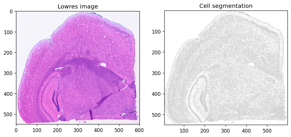
Use spatialdata-plot to visualize tissue morphology:

%%time
axes = plt.subplots(1, 2, figsize=(10, 5))[1].flatten()
sdata.pl.render_images(f"{dataset_id}_lowres_image").pl.show(
    coordinate_systems=f"{dataset_id}_downscaled_lowres",
    ax=axes[0], title="Lowres image"
)
sdata.pl.render_shapes(f"{dataset_id}_cell_segmentations").pl.show(
    coordinate_systems=f"{dataset_id}_downscaled_lowres",
    ax=axes[1], title="Cell segmentation"
)

Clipping input data to the valid range for imshow with RGB data ([0..1] for floats or [0..255] for integers). Got range [-0.1658031..1.0].

INFO     Using 'datashader' backend with 'None' as reduction method to speed up plotting. Depending on the         
         reduction method, the value range of the plot might change. Set method to 'matplotlib' to disable this    
         behaviour.                                                                                                
CPU times: user 4.43 s, sys: 182 ms, total: 4.61 s
Wall time: 4.92 s

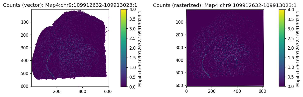
To visualize peak expression as an image, rasterize the spatial bins first:

%%time
for bin_size in ["016", "008", "002"]:
    # rasterize_bins() requires a compressed sparse column (csc) matrix
    sdata.tables[f"square_{bin_size}um"].X = sdata.tables[f"square_{bin_size}um"].X.tocsc()
    rasterized = rasterize_bins(
        sdata,
        f"{dataset_id}_square_{bin_size}um",
        f"square_{bin_size}um",
        "array_col",
        "array_row",
    )
    sdata[f"rasterized_{bin_size}um"] = rasterized

CPU times: user 6.48 s, sys: 1.72 s, total: 8.2 s
Wall time: 9.11 s

Then visualize a peak’s global expression at 16µm resolution:

%%time
peak_name = 'Map4:chr9:109912632-109913023:1'
print(f"Using example feature: {peak_name}")

axes = plt.subplots(1, 2, figsize=(10, 5))[1].flatten()
sdata.pl.render_shapes(f"{dataset_id}_square_016um", color=peak_name).pl.show(
    coordinate_systems=f"{dataset_id}_downscaled_lowres",
    ax=axes[0], title=f"Counts (vector): {peak_name}"
)
sdata.pl.render_images(f"rasterized_016um", channel=peak_name).pl.show(
    coordinate_systems=f"{dataset_id}_downscaled_lowres",
    ax=axes[1], title=f"Counts (rasterized): {peak_name}"
)
plt.subplots_adjust(wspace=1)
plt.show()

Using example feature: Map4:chr9:109912632-109913023:1
INFO     Using 'datashader' backend with 'None' as reduction method to speed up plotting. Depending on the         
         reduction method, the value range of the plot might change. Set method to 'matplotlib' to disable this    
         behaviour.                                                                                                
INFO     Using the datashader reduction "mean". "max" will give an output very close to the matplotlib result.     

CPU times: user 10.2 s, sys: 3.69 s, total: 13.9 s
Wall time: 16.1 s

Spatial variability testing with SplisosmFFT

To detect peak usage variation within a given gene, we run spatial variability test using hsic-ir.

Data filtering and model setup

Peak filtering criteria:

• min_counts: minimum total UMI count across all bins.

• min_bin_pct: minimum fraction of bins in which a peak must be detected.

• Genes with fewer than two passing peaks are automatically excluded.

model = SplisosmFFT(neighbor_degree=1, rho=0.99)
model.setup_data(
    sdata=sdata,
    bins=test_bins_element,
    table_name=test_table,
    col_key="array_col",
    row_key="array_row",
    layer="counts",
    group_iso_by=group_iso_by, # 'gene_ids'
    gene_names=gene_name_col, # 'gene_ids'
    min_counts=min_counts,
    min_bin_pct=min_bin_pct,
)
print(model)

=== FFT SPLISOSM model for spatial isoform testings
- Number of genes: 1061
- Number of observed spots: 94592
- Number of raster cells: 134688
- Average number of isoforms per gene: 2.226201696512724
=== Test results
- Spatial variability test: NA
- Differential usage test: NA

Extract gene-level summary statistics:

%%time
gene_meta = model.extract_feature_summary(level='gene')
gene_meta.sort_values('perplexity', ascending=False).head(5)

Genes: 100%|██████████| 1061/1061 [00:01<00:00, 634.64it/s]

CPU times: user 1.78 s, sys: 195 ms, total: 1.97 s
Wall time: 2.01 s

	n_isos	perplexity	pct_bin_on	count_avg	count_std
gene
Ppp3ca	6	4.951889	0.407138	0.869429	1.597794
Celf4	5	3.819581	0.202174	0.250539	0.552908
Homer1	4	3.788384	0.063769	0.070535	0.283515
Pcmt1	4	3.785652	0.139145	0.161441	0.432617
Rbbp6	4	3.780505	0.081297	0.087640	0.305624

Peak-level summary is also available:

peak_meta = model.extract_feature_summary(level='isoform')
peak_meta.sort_values('gene_ids', ascending=False).head(5)

	gene_ids	probe_ids	feature_types	CDS	Junctions	UTR3	UTR5	end	exon	genome	...	start	strand	width	pct_bin_on	count_total	count_avg	count_std	ratio_total	ratio_avg	ratio_std
mt-Nd5:chrM:12597-13503:1	mt-Nd5	mt-Nd5:chrM:12597-13503:1	Gene Expression	YES	no-junctions			13503	YES		...	12597	+	907	0.295427	35035.0	0.370380	0.642801	0.672909	0.670371	0.432255
mt-Nd5:chrM:11870-13196:1	mt-Nd5	mt-Nd5:chrM:11870-13196:1	Gene Expression	YES	no-junctions			13196	YES		...	11870	+	1327	0.135720	14026.0	0.148279	0.391148	0.269394	0.271458	0.408964
mt-Nd5:chrM:11742-12338:1	mt-Nd5	mt-Nd5:chrM:11742-12338:1	Gene Expression	YES	no-junctions			12338	YES		...	11742	+	597	0.031123	3004.0	0.031757	0.178934	0.057697	0.058170	0.215502
mt-Nd4:chrM:11161-11413:1	mt-Nd4	mt-Nd4:chrM:11161-11413:1	Gene Expression	YES	no-junctions			11413	YES		...	11161	+	253	0.906726	332118.0	3.511058	2.643438	0.937358	0.936997	0.150768
mt-Nd4:chrM:11100-11519:1	mt-Nd4	mt-Nd4:chrM:11100-11519:1	Gene Expression	YES	across-junctions			11519	YES		...	11100	+	420	0.168820	17843.0	0.188631	0.443044	0.050359	0.050763	0.136139

5 rows × 22 columns

Running spatial variability test

%%time

model.test_spatial_variability(
    method="hsic-ir",
    ratio_transformation="none",
    n_jobs=-1,
    print_progress=True,
)
sv_res_16um = model.get_formatted_test_results("sv").sort_values("pvalue_adj")

SV (hsic-ir): 100%|██████████| 1061/1061 [00:17<00:00, 59.14it/s]

CPU times: user 32.9 s, sys: 6.55 s, total: 39.5 s
Wall time: 18.2 s

Top genes, sorted by adjusted p-value:

sig_001 = int((sv_res_16um["pvalue_adj"] < 0.01).sum())
print(
    "Spatially variably processed genes (FDR < 0.01, 16um): "
    f"{sig_001} out of {sv_res_16um.shape[0]} total genes"
)
sv_res_16um.head(5)

Spatially variably processed genes (FDR < 0.01, 16um): 501 out of 1061 total genes

	gene	statistic	pvalue	pvalue_adj
357	Gls	6.126092e-07	0.0	0.0
293	Ensa	1.468206e-06	0.0	0.0
340	Gabbr1	2.055658e-06	0.0	0.0
77	Arpp21	2.619232e-06	0.0	0.0
85	Atp1b1	2.350605e-06	0.0	0.0

Merge gene-level summary back into results:

sv_res_16um.merge(
    gene_meta.reset_index()[['gene', 'n_isos', 'perplexity', 'pct_bin_on']],
    on='gene',
    how='left',
).head(5)

	gene	statistic	pvalue	pvalue_adj	n_isos	perplexity	pct_bin_on
0	Gls	6.126092e-07	0.0	0.0	2	1.514386	0.124408
1	Ensa	1.468206e-06	0.0	0.0	3	2.289981	0.177774
2	Gabbr1	2.055658e-06	0.0	0.0	4	2.846700	0.229692
3	Arpp21	2.619232e-06	0.0	0.0	4	2.701563	0.154178
4	Atp1b1	2.350605e-06	0.0	0.0	4	2.129971	0.463348

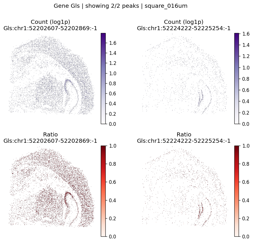
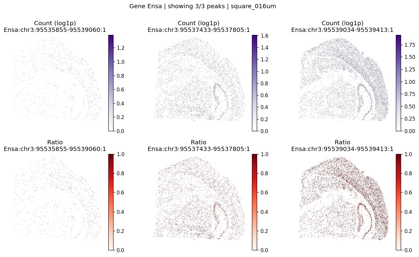
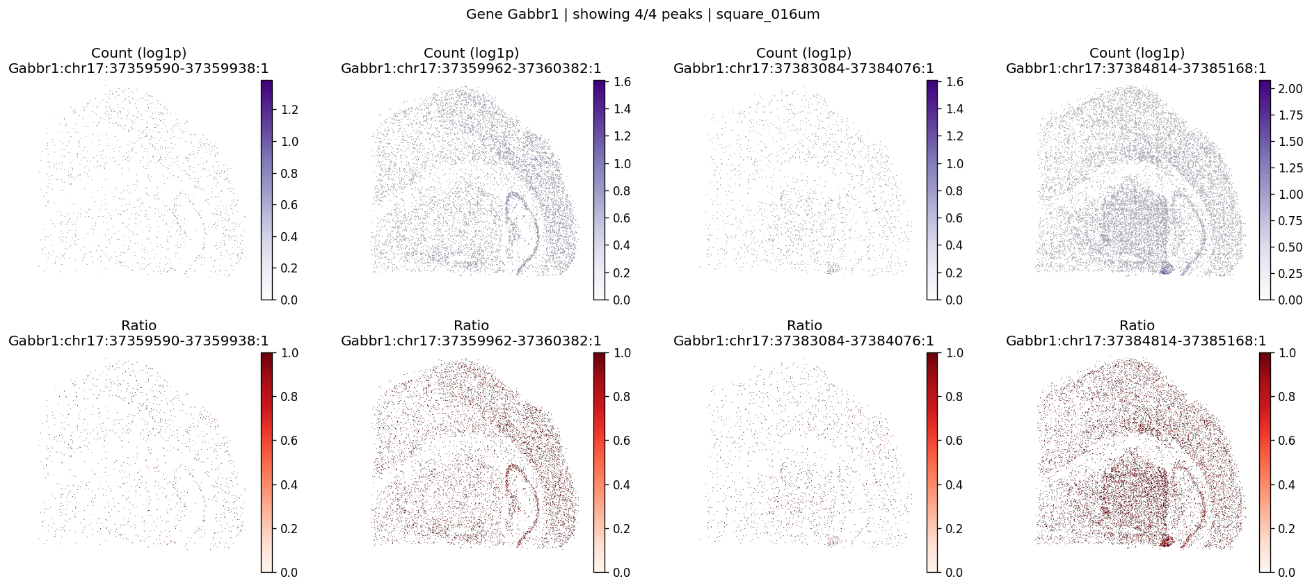
Visualize significant events

The helper below renders per-peak log1p counts and within-gene ratios on the testing grid.

def ensure_rasterized(sdata, bin_table: str, bin_element: str, layer: str = "counts"):
    raster_key = f"rasterized_{bin_table}_{layer}"
    if raster_key in sdata.images:
        return raster_key

    adata = sdata.tables[bin_table]
    adata.X = adata.layers[layer]
    if hasattr(adata.X, "tocsc") and getattr(adata.X, "format", None) != "csc":
        adata.X = adata.X.tocsc()

    sdata[raster_key] = rasterize_bins(
        sdata,
        bins=bin_element,
        table_name=bin_table,
        col_key="array_col",
        row_key="array_row",
    )
    return raster_key

The plotting function checks peak availability, lazily rasterizes data on demand, computes log1p counts and within-gene ratios, and optionally masks zero values.

def plot_gene_peak_maps(
    sdata,
    bin_table: str,
    bin_element: str,
    gene_id: str,
    peak_meta: pd.DataFrame | None = None,
    group_col: str = "gene_ids",
    max_peaks: int = 4,
    hide_zero_count: bool = True,
    hide_zero_ratio: bool = True,
):
    adata = sdata.tables[bin_table]
    if peak_meta is None:
        peak_meta = adata.var.copy()

    if group_col not in peak_meta.columns:
        raise ValueError(f"'{group_col}' not found in peak_meta columns")

    peak_names = peak_meta.index[
        peak_meta[group_col].astype(str) == str(gene_id)
    ].tolist()
    if len(peak_names) == 0:
        raise ValueError(f"No peaks found for gene id '{gene_id}'")
    if any(peak not in adata.var_names for peak in peak_names):
        raise ValueError(f"Some peaks not found in {bin_table}.var_names")
    n_peaks = len(peak_names)
    n_shown = min(n_peaks, max_peaks)
    peak_names = peak_names[:n_shown]

    raster_key = ensure_rasterized(sdata, bin_table=bin_table, bin_element=bin_element)
    data = sdata[raster_key].sel(c=peak_names).values
    counts_cube = np.moveaxis(np.asarray(data, dtype=float), 0, -1)

    counts_flat = counts_cube.reshape(-1, counts_cube.shape[-1])
    ratios_flat = counts_to_ratios(counts_flat, transformation="none", nan_filling="none")
    ratios_cube = ratios_flat.numpy().reshape(counts_cube.shape)

    n_peak = counts_cube.shape[-1]
    fig, axes = plt.subplots(2, n_peak, figsize=(4 * n_peak, 7), squeeze=False)

    for i, peak in enumerate(peak_names):
        c = counts_cube[:, :, i]
        r = ratios_cube[:, :, i]
        if hide_zero_count:
            c = np.where(c == 0, np.nan, c)
        if hide_zero_ratio:
            r = np.where(r == 0, np.nan, r)

        im0 = axes[0, i].imshow(np.log1p(c), cmap="Purples", vmin=0.0)
        axes[0, i].set_title(f"Count (log1p)\n{peak}")
        axes[0, i].axis("off")
        fig.colorbar(im0, ax=axes[0, i], fraction=0.046, pad=0.04)

        vmax = np.nanpercentile(ratios_cube, 99) if np.isfinite(ratios_cube).any() else 1.0
        im1 = axes[1, i].imshow(r, cmap="Reds", vmin=0.0, vmax=vmax)
        axes[1, i].set_title(f"Ratio\n{peak}")
        axes[1, i].axis("off")
        fig.colorbar(im1, ax=axes[1, i], fraction=0.046, pad=0.04)

    fig.suptitle(f"Gene {gene_id} | showing {n_shown}/{n_peaks} peaks | {bin_table}", y=1)
    fig.tight_layout()
    plt.show()

top_genes = sv_res_16um.head(10)["gene"].astype(str).tolist()
top_genes[:5]

['Gls', 'Ensa', 'Gabbr1', 'Arpp21', 'Atp1b1']

for gene_id in top_genes[:3]:
    plot_gene_peak_maps(
        sdata=sdata,
        bin_table=test_table,
        bin_element=test_bins_element,
        gene_id=gene_id,
        group_col='gene_ids',
        max_peaks=6,
        peak_meta=peak_meta,
        hide_zero_ratio=True,
    )

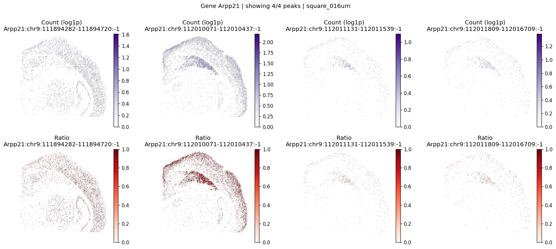
%%time
# Example: inspect a specific gene manually
plot_gene_peak_maps(
    sdata, test_table, test_bins_element, 
    gene_id="Arpp21", 
    group_col='gene_ids', 
    peak_meta=peak_meta
)

CPU times: user 444 ms, sys: 36.3 ms, total: 480 ms
Wall time: 484 ms

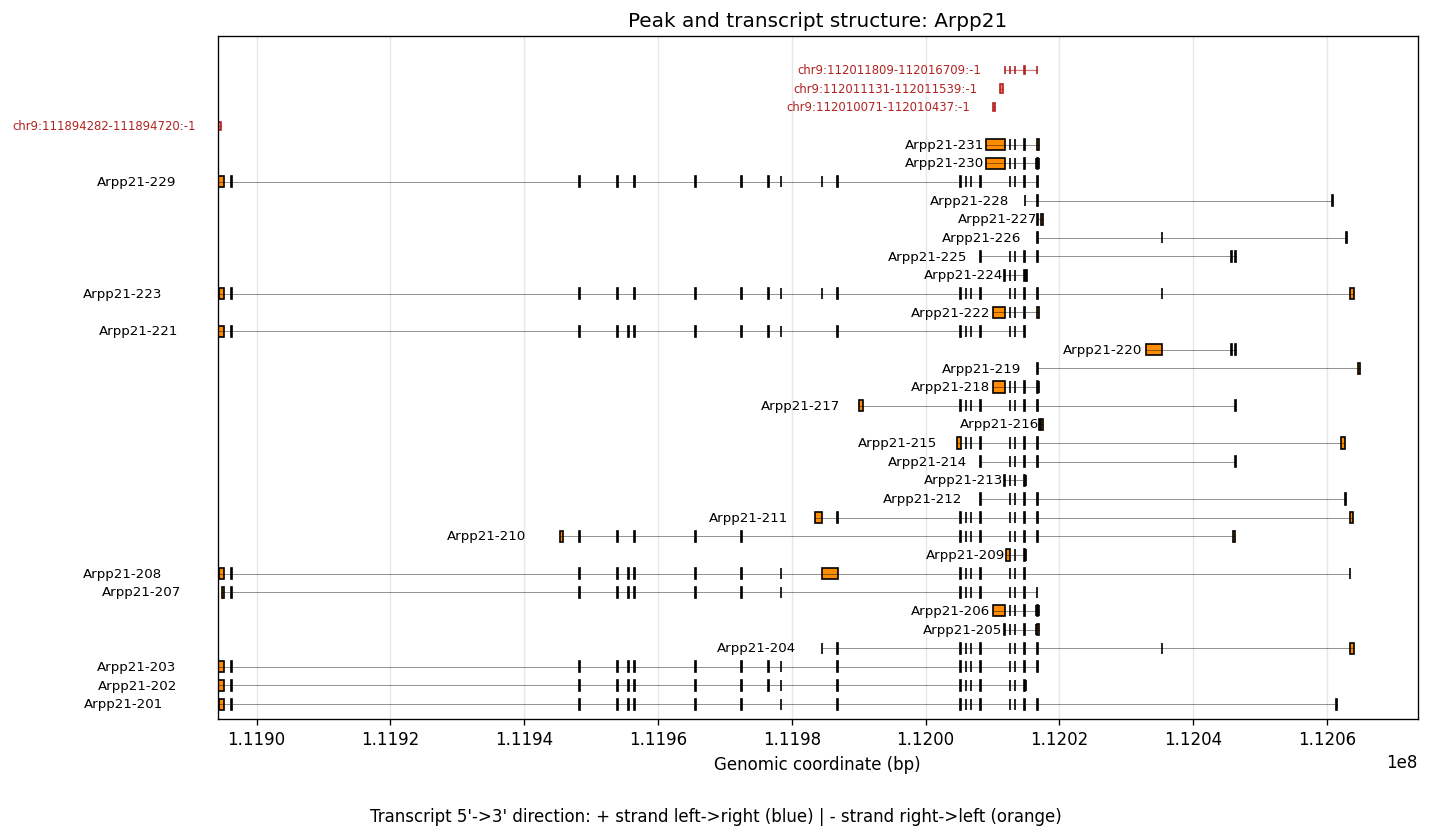
To see the spatially variable transcript regions, we can visualize TREND peaks along with a matched transcript reference. The following files need to be downloaded and provided as input:

• peak.txt.bed12 from the Sierra peak calling output (see scripts/visiumhd_3p_trend_quant.sh for details)

• gencode.vM33.annotation.gtf.gz from GENCODE

Show code cell source

Hide code cell source

def plot_peak_transcript_structure(
    gene_name: str,
    bed12_file: str | Path,
    gtf_file: str | Path,
    figsize: tuple[float, float] = (12, 7),
    transcript_label: str = "transcript_name",
):
    """Visualize BED12 peaks and transcript exon structure for one gene.

    The BED12 peak model is rendered with block-level segments, and transcript
    structures are drawn in the same style as plot_probe_transcript_structure:
    introns as thin lines and exons as thicker boxes with transcript labels.
    """
    import gzip

    bed12_file = Path(bed12_file)
    gtf_file = Path(gtf_file)

    # BED12 schema used by Sierra peak output.
    bed_cols = [
        "chrom", "start", "end", "name", "score", "strand",
        "thickStart", "thickEnd", "itemRgb", "blockCount", "blockSizes", "blockStarts",
    ]
    peaks = pd.read_csv(
        bed12_file,
        sep="\t",
        header=None,
        names=bed_cols,
        usecols=list(range(12)),
    )

    # Parse peak name format: GENE:chr:start-end:strand
    peaks["gene"] = peaks["name"].astype(str).str.split(":", n=1).str[0]
    peaks["peak_id"] = peaks["name"].astype(str).str.split(":", n=1).str[1]
    peaks["peak_id"] = peaks["peak_id"].fillna(peaks["name"])

    peaks = peaks[peaks["gene"].str.lower() == str(gene_name).lower()].copy()
    if peaks.empty:
        warnings.warn(f"No BED12 peaks found for gene '{gene_name}' in {bed12_file}")

    # Convert BED12 blocks to absolute genomic coordinates per peak.
    def parse_blocks(row: pd.Series) -> list[tuple[int, int]]:
        starts = [int(x) for x in str(row["blockStarts"]).strip(",").split(",") if x != ""]
        sizes = [int(x) for x in str(row["blockSizes"]).strip(",").split(",") if x != ""]
        n = min(int(row["blockCount"]), len(starts), len(sizes))
        blocks = []
        for i in range(n):
            block_start = int(row["start"]) + starts[i]
            block_end = block_start + sizes[i]
            blocks.append((block_start, block_end))
        return blocks

    if not peaks.empty:
        peaks["blocks"] = peaks.apply(parse_blocks, axis=1)

    # Open plain-text or gzipped GTF seamlessly.
    if str(gtf_file).endswith(".gz"):
        gtf_opener = lambda f: gzip.open(f, "rt")
    else:
        gtf_opener = open

    # Collect exon structures keyed by transcript_id.
    transcripts_by_id = {}
    with gtf_opener(gtf_file) as f:
        for line in f:
            if line.startswith("#"):
                continue
            fields = line.rstrip("\n").split("\t")
            if len(fields) < 9 or fields[2] != "exon":
                continue

            start, end = int(fields[3]), int(fields[4])
            attrs = {}
            for attr in fields[8].split(";"):
                attr = attr.strip()
                if not attr or " " not in attr:
                    continue
                k, v = attr.split(" ", 1)
                attrs[k] = v.strip().strip('"')

            if attrs.get("gene_name", "").lower() != str(gene_name).lower() and attrs.get("gene_id", "").lower() != str(gene_name).lower():
                continue

            tx_id = attrs.get("transcript_id", "unknown")
            if tx_id not in transcripts_by_id:
                tx_name = attrs.get(transcript_label) or attrs.get("transcript_name") or tx_id
                transcripts_by_id[tx_id] = {
                    "tx_name": tx_name,
                    "strand": fields[6],
                    "exons": [],
                }
            transcripts_by_id[tx_id]["exons"].append((start, end))

    if not transcripts_by_id:
        warnings.warn(f"No matching transcripts found for gene '{gene_name}' in {gtf_file}")

    fig, ax = plt.subplots(figsize=figsize)

    y_pos = 0
    x_mins = []
    x_maxs = []

    # Strand color coding for cleaner direction cues.
    strand_colors = {
        "+": "steelblue",
        "-": "darkorange",
    }

    # Draw transcripts first using the same visual language as probe plotting.
    for tx_id, tx_info in sorted(transcripts_by_id.items()):
        exons = sorted(tx_info["exons"])
        if not exons:
            continue

        min_coord = min(e[0] for e in exons)
        max_coord = max(e[1] for e in exons)
        x_mins.append(min_coord)
        x_maxs.append(max_coord)

        strand = str(tx_info.get("strand", "."))
        tx_color = strand_colors.get(strand, "gray")

        # Introns: thin baseline
        ax.plot([min_coord, max_coord], [y_pos, y_pos], "k-", linewidth=0.5, alpha=0.5)

        # Exons: thicker boxes (color by strand)
        for exon_start, exon_end in exons:
            ax.barh(
                y_pos,
                exon_end - exon_start,
                left=exon_start,
                height=0.6,
                color=tx_color,
                edgecolor="black",
            )

        # Transcript label (same style as probe-based helper)
        tx_name = str(tx_info.get("tx_name", tx_id))
        ax.text(
            min_coord - (max_coord - min_coord) * 0.05,
            y_pos,
            tx_name[:30],
            ha="right",
            va="center",
            fontsize=8,
        )

        y_pos += 1

    # Plot peaks after transcripts, one row per peak to avoid overlap.
    peak_rows_start = y_pos
    peak_rows = peaks.sort_values(["chrom", "start", "end"]) if not peaks.empty else peaks

    for i, (_, row) in enumerate(peak_rows.iterrows()):
        peak_y = peak_rows_start + i
        blocks = row["blocks"] if isinstance(row["blocks"], list) and row["blocks"] else [(int(row["start"]), int(row["end"]))]
        peak_min = min(b[0] for b in blocks)
        peak_max = max(b[1] for b in blocks)
        x_mins.append(peak_min)
        x_maxs.append(peak_max)

        # Span and block model for each peak.
        ax.plot([peak_min, peak_max], [peak_y, peak_y], color="firebrick", linewidth=0.7, alpha=0.6)
        for block_start, block_end in blocks:
            ax.barh(
                peak_y,
                block_end - block_start,
                left=block_start,
                height=0.45,
                color="salmon",
                edgecolor="firebrick",
            )

    x_pad = max(1.0, (max(x_maxs) - min(x_mins)) * 0.02) if x_mins and x_maxs else 1.0

    # Peak labels are shown on the left side, one per row.
    for i, (_, row) in enumerate(peak_rows.iterrows()):
        peak_y = peak_rows_start + i
        blocks = row["blocks"] if isinstance(row["blocks"], list) and row["blocks"] else [(int(row["start"]), int(row["end"]))]
        peak_min = min(b[0] for b in blocks)
        ax.text(
            peak_min - x_pad,
            peak_y,
            str(row["peak_id"]),
            va="center",
            ha="right",
            fontsize=7,
            color="firebrick",
        )

    total_rows = max(y_pos, peak_rows_start + len(peak_rows))
    ax.set_ylim(-0.8, total_rows + 0.8)
    ax.set_yticks([])
    ax.set_xlabel("Genomic coordinate (bp)")
    ax.set_title(f"Peak and transcript structure: {gene_name}")
    ax.grid(True, axis="x", alpha=0.3)

    # Place strand direction note as a single centered row below the plot.
    direction_note = "Transcript 5'->3' direction: + strand left->right (blue) | - strand right->left (orange)"
    fig.text(0.5, 0.01, direction_note, ha="center", va="bottom", fontsize=10, color="black")

    # Reserve bottom margin for the legend row.
    fig.tight_layout(rect=(0.0, 0.05, 1.0, 1.0))
    plt.show()

%%time
plot_peak_transcript_structure(
    gene_name="Arpp21",
    bed12_file="/Users/jysumac/Projects/SPLISOSM_paper/data/visiumhd_3p_mouse_cbs/sierra_peaks/peak.txt.bed12",
    gtf_file="/Users/jysumac/reference/mm39/gencode.vM33.annotation.gtf.gz",
)

CPU times: user 7.01 s, sys: 42.8 ms, total: 7.06 s
Wall time: 7.19 s

Advanced analyses

Spatial resolution comparison

For illustration, we use the top 200 genes from the 16µm analysis as the reference set:

# np.random.seed(42)
# gene_names = sdata.tables[test_table].var['gene_ids'].unique()
# gene_subset = np.random.choice(gene_names, size=500, replace=False)
gene_subset = sv_res_16um.sort_values('pvalue').head(500)['gene'].astype(str).tolist()

Run spatial variability tests across all three resolutions:

%%time
# Compare results across 2µm, 8µm, 16µm resolutions
resolutions = [
    {'bin': f'{dataset_id}_square_002um', 'table_name': 'square_002um'},
    {'bin': f'{dataset_id}_square_008um', 'table_name': 'square_008um'},
    {'bin': f'{dataset_id}_square_016um', 'table_name': 'square_016um'},
]

res_results = []
for res in resolutions:
    m = SplisosmFFT(neighbor_degree=1, rho=0.99)
    sdata_subset = sd.filter_by_table_query(
        sdata,
        table_name=res['table_name'],
        var_expr=an.col(gene_name_col).is_in(gene_subset),
    )
    m.setup_data(
        sdata_subset,
        bins=res['bin'],
        table_name=res['table_name'],
        col_key="array_col",
        row_key="array_row",
        layer="counts",
        group_iso_by=group_iso_by,
        gene_names=gene_name_col,
        min_counts=min_counts,
        min_bin_pct=0.0
    )
    m.test_spatial_variability(method='hsic-ir')
    results = m.get_formatted_test_results('sv')[['gene', 'pvalue']].copy()
    results.rename(columns={'pvalue': f"p_{res['table_name']}"}, inplace=True)
    res_results.append(results)

SV (hsic-ir): 100%|██████████| 500/500 [19:46<00:00,  2.37s/it]
SV (hsic-ir): 100%|██████████| 500/500 [00:21<00:00, 23.43it/s]
SV (hsic-ir): 100%|██████████| 500/500 [00:07<00:00, 68.97it/s]

CPU times: user 24min 30s, sys: 31min 2s, total: 55min 33s
Wall time: 21min 10s

merged = res_results[0]
for res in res_results[1:]:
    merged = merged.merge(res, on="gene", how="inner")

p_cols = [c for c in merged.columns if c.startswith("p_")]
print("Spearman correlation across spatial resolutions:")
display(merged[p_cols].corr(method="spearman"))

Spearman correlation across spatial resolutions:

	p_square_002um	p_square_008um	p_square_016um
p_square_002um	1.000000	0.755450	0.625206
p_square_008um	0.755450	1.000000	0.901805
p_square_016um	0.625206	0.901805	1.000000

pairs = list(combinations(p_cols, 2))
if pairs:
    fig, axes = plt.subplots(1, len(pairs), figsize=(3 * len(pairs), 3), squeeze=False)
    axes = axes.ravel()

    for ax, (x_col, y_col) in zip(axes, pairs):
        x = merged[x_col].to_numpy()
        y = merged[y_col].to_numpy()
        corr, pval = spearmanr(x, y)

        ax.scatter(x + 1e-300, y + 1e-300, s=8, alpha=0.5)
        ax.set_xscale("log")
        ax.set_yscale("log")
        ax.set_xlabel(x_col)
        ax.set_ylabel(y_col)
        ax.set_title(f"Spearman ρ={corr:.3f}")
        ax.grid(True, alpha=0.3)

        low = 1e-300
        high = max(np.max(x), np.max(y))
        ax.plot([low, high], [low, high], "r--", alpha=0.5, linewidth=1.5)
        ax.set_xlim(low, high)
        ax.set_ylim(low, high)

    plt.tight_layout()
    plt.show()

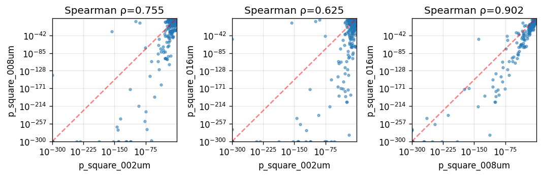
Gene rankings are broadly consistent across resolutions, especially between 16µm and 8µm. The 2µm analysis shows stronger statistical significance, likely because the kernel places more weight on low-frequency patterns at finer scales.

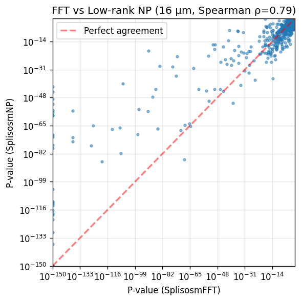
Method comparison: SplisosmFFT vs SplisosmNP

Compare FFT-accelerated and non-parametric spatial variability tests at 16 µm resolution.

SplisosmNP.setup_data performs low-rank kernel approximation (controlled by approx_rank). A higher rank gives more accurate approximations at increased cost. Here we use approx_rank=20 for demonstration.

%%time
# Run SplisosmNP at 16µm for direct comparison with SplisosmFFT
model_np = SplisosmNP()
model_np.setup_data(
    adata=sdata.tables[test_table],
    spatial_key='spatial', # adata.obsm key for spatial coordinates
    layer='counts',
    approx_rank=20,
    group_iso_by=group_iso_by, # 'gene_ids'
    gene_names=gene_name_col, # 'gene_ids'
    min_counts=min_counts,
    min_bin_pct=min_bin_pct,
)

CPU times: user 2min 4s, sys: 6.09 s, total: 2min 10s
Wall time: 1min 15s

%%time
model_np.test_spatial_variability(
    method='hsic-ir',
    ratio_transformation='none',
    print_progress=True,
)

100%|██████████| 1061/1061 [00:02<00:00, 397.27it/s]

CPU times: user 3.9 s, sys: 498 ms, total: 4.4 s
Wall time: 2.68 s

Compare p-values between SplisosmFFT and SplisosmNP:

# Extract results and merge
sv_np = model_np.get_formatted_test_results('sv')[['gene', 'pvalue']].copy()
sv_np = sv_np.rename(columns={'pvalue': 'pvalue_np'})

comparison = sv_res_16um[['gene', 'pvalue']].copy()
comparison = comparison.rename(columns={'pvalue': 'pvalue_fft'})
comparison = comparison.merge(sv_np, on='gene', how='inner')

corr, _ = spearmanr(comparison['pvalue_fft'], comparison['pvalue_np'])

print(f'Genes tested in both methods: {len(comparison)}')
print(f'== Significant in SplisosmFFT (FDR < 0.01): {(comparison["pvalue_fft"] < 0.01).sum()}')
print(f'== Significant in SplisosmNP (FDR < 0.01): {(comparison["pvalue_np"] < 0.01).sum()}')
print(f'== P-value correlation (Spearman rho): {corr:.4f}')

Genes tested in both methods: 1061
== Significant in SplisosmFFT (FDR < 0.01): 537
== Significant in SplisosmNP (FDR < 0.01): 620
== P-value correlation (Spearman rho): 0.7945

# Scatter plot comparison
fig, ax = plt.subplots(figsize=(5, 5))
x = comparison['pvalue_fft'].to_numpy()
y = comparison['pvalue_np'].to_numpy()

ax.scatter(x + 1e-150, y + 1e-150, s=8, alpha=0.5)
ax.set_xscale('log')
ax.set_yscale('log')
ax.set_xlabel('P-value (SplisosmFFT)')
ax.set_ylabel('P-value (SplisosmNP)')
ax.set_title(f'FFT vs Low-rank NP (16 µm, Spearman ρ={corr:.2f})')
ax.grid(True, alpha=0.3)

# Add diagonal reference line
lims = [1e-150, 1.0]
ax.plot(lims, lims, 'r--', alpha=0.5, label='Perfect agreement', linewidth=2)
ax.legend()
ax.set_xlim(lims)
ax.set_ylim(lims)

plt.tight_layout()
plt.show()

Summary and recommendations

Key findings:

1. Spatial variability is robustly detectable in this Visium HD 3’ peak-level dataset using SplisosmFFT on regular grids.

2. Spatial resolution trade-offs:

   • 16 um: Fast and reliable - recommended for initial exploration.

   • 8 um: High agreement with 16 um results.

   • 2 um: Highest resolution but slower and sparser.

3. Method equivalence: SplisosmFFT and SplisosmNP yield concordant rankings on regular grids, particularly for genes with strong spatial patterns.

Recommendations:

• Start with 16 um binning for exploratory analysis.

• Refine with 8 um if finer spatial detail is needed.

• Use SplisosmFFT on regular grids (Visium HD, Xenium binned data) with neighbor_degree=1, rho=0.99 as a robust default.

• Use SplisosmNP for irregular geometries (e.g., cell-segmented data).

For reproducibility

import sys
from datetime import date
import splisosm

print("Last updated:", date.today())
print("Python:", sys.version.split()[0])
print("splisosm:", getattr(splisosm, "__version__", "unknown"))

Last updated: 2026-03-17
Python: 3.12.12
splisosm: 1.0.4