Single-cell segmented data (Xenium Prime 5K)

This notebook demonstrates how to run SPLISOSM’s spatial variability and differential usage tests on single-cell segmented spatial transcriptomics data, using the 10x Genomics Xenium Prime 5K Mouse Brain Coronal dataset as an example. Because cell centroids are not on a regular grid, SplisosmFFT does not apply; we use SplisosmNP instead. The following analyses are performed:

1. Run spatial variability (SV) tests to identify spatially variable processed (SVP) genes with variable codeword usage, including on a per-cluster basis (within cell-type variability).

2. Compare two null distribution methods — 'eig' (Liu’s chi-square mixture, with low-rank approximation) vs 'welch'/'clt' (moment-matching approximation).

3. Run differential isoform usage (DU) test to find cluster-specific codeword usage switches, as well as SVP usage associations with RBP (RNA-binding protein) expression.

4. Run variability tests using an expression-based k-NN graph to identify genes with variable codeword usage across cell states.

Estimated runtime: ~15 min.

Preliminary notes

For Xenium Prime 5K datasets, each gene is profiled by multiple codewords (i.e., exon/junction probe sets). This notebook uses the same Xenium dataset as presented in the SPLISOSM paper and as in the SplisosmFFT Xenium Prime 5K tutorial.

• The dataset can be downloaded from 10x Genomics here

• Probe set (5K Mouse Pan Tissue and Pathways Panel) information is available here.

Cell-segmentation was performed as part of the Xenium Onboard Analysis. After downloading Xenium analysis outputs, we reran the Xenium Ranger v3.1.0 relabel pipeline to get codeword transcript counts. Due to Xenium output data structure changes, if you encounter issues, consider re-running the Xenium Ranger (v3.1.0+) relabel pipeline as well. See 10x documentation for guidance.

Imports

from pathlib import Path
from scipy.stats import spearmanr
import numpy as np
import pandas as pd
import scanpy as sc
import matplotlib.pyplot as plt

from splisosm import SplisosmNP
from splisosm.utils import add_ratio_layer
from splisosm.io import load_xenium_codeword

# set random seed for reproducibility
np.random.seed(0)

Configure paths and core parameters

# Required: Xenium Ranger output directory (either the `outs` dir itself or its parent)
xenium_prime_outs = Path('/path/to/xenium_prime_5k/outs')

# Feature grouping and filters
group_iso_by = 'gene_symbol'
gene_name_col = 'gene_symbol'
min_counts = 50
min_bin_pct = 0.01

# Xenium transcript filter
quality_threshold = 20.0

Load single-cell segmented data

We use splisosm.io.load_xenium_codeword to load the cell-by-gene and cell-by-codeword count matrices from Xenium outputs and relevant metadata as a SpatialData object.

• spatial_resolutions=[] disables spatial binning

• build_cell_codeword_table=True loads the cell-by-codeword AnnData as well as the cell-by-gene AnnData.

%%time
print('Building Xenium codeword SpatialData from transcript chunks...')
sdata = load_xenium_codeword(
    path=xenium_prime_outs,
    spatial_resolutions=[], # or None to skip binning
    quality_threshold=quality_threshold,
    counts_layer_name='counts',
    build_cell_codeword_table=True, # also build cell-by-codeword table
    transcripts=False, # skip transcript-level points
    n_jobs=1
)

sdata

Building Xenium codeword SpatialData from transcript chunks...

/Users/jysumac/miniforge3/envs/splisosm_dev/lib/python3.12/functools.py:912: ImplicitModificationWarning: Transforming to str index.
  return dispatch(args[0].__class__)(*args, **kw)

CPU times: user 50.2 s, sys: 14.9 s, total: 1min 5s
Wall time: 26.4 s

SpatialData object
├── Images
│     └── 'morphology_focus': DataTree[cyx] (4, 23912, 34154), (4, 11956, 17077), (4, 5978, 8538), (4, 2989, 4269), (4, 1494, 2134)
├── Labels
│     ├── 'cell_labels': DataTree[yx] (23912, 34154), (11956, 17077), (5978, 8538), (2989, 4269), (1494, 2134)
│     └── 'nucleus_labels': DataTree[yx] (23912, 34154), (11956, 17077), (5978, 8538), (2989, 4269), (1494, 2134)
├── Shapes
│     ├── 'cell_boundaries': GeoDataFrame shape: (63173, 1) (2D shapes)
│     └── 'nucleus_boundaries': GeoDataFrame shape: (63036, 1) (2D shapes)
└── Tables
      ├── 'table': AnnData (63173, 5006)
      └── 'table_codeword': AnnData (63173, 11163)
with coordinate systems:
    ▸ 'global', with elements:
        morphology_focus (Images), cell_labels (Labels), nucleus_labels (Labels), cell_boundaries (Shapes), nucleus_boundaries (Shapes)

There are two anndata objects associated with this dataset:

• sdata.tables['table']: cell-by-gene counts (default loaded by spatialdata-io)

• sdata.tables['table_codeword']: cell-by-codeword counts. Cell centroid spatial coordinates are stored in adata.obsm['spatial'].

adata_gene = sdata.tables['table']
adata_codeword = sdata.tables['table_codeword']
print(f"=== Number of cells: {adata_codeword.shape[0]} ===")
print(f"=== Number of genes: {adata_gene.shape[1]} ===")
print(f"=== Number of codewords: {adata_codeword.shape[1]} ===")

=== Number of cells: 63173 ===
=== Number of genes: 5006 ===
=== Number of codewords: 11163 ===

Expression-based clustering

We first run the standard Scanpy preprocessing and clustering pipeline to get gene-expression-based cell clusters. Similar to differentially expressed gene markers, we can also identify genes with differential codeword usage across clusters using Splisosm’s DU test (to be described later).

%%time
# set obs_name to cell_id
adata_gene.obs.set_index('cell_id', inplace=True)

# log-normalization
adata_gene.layers['counts'] = adata_gene.X.copy()
sc.pp.normalize_total(adata_gene, target_sum=1e4)
sc.pp.log1p(adata_gene)
adata_gene.layers['log1p'] = adata_gene.X.copy()

# dimensionality reduction
sc.pp.highly_variable_genes(adata_gene, n_top_genes=2000, layer='log1p')
sc.pp.pca(adata_gene, n_comps=50, use_highly_variable=True, layer='log1p')

<timed exec>:6: UserWarning: Some cells have zero counts

CPU times: user 4.34 s, sys: 232 ms, total: 4.57 s
Wall time: 4.47 s

%%time
# neighborhood graph and UMAP
sc.pp.neighbors(adata_gene, n_neighbors=15)
sc.tl.umap(adata_gene)

# clustering
sc.tl.leiden(adata_gene, flavor="igraph", n_iterations=2, resolution=0.5)

CPU times: user 34.4 s, sys: 577 ms, total: 35 s
Wall time: 35.1 s

with plt.rc_context({"figure.figsize": (3, 3)}):
    sc.pl.umap(adata_gene, color=["leiden"])

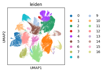
In addition to the cell annotation, we also get an expression-based symmetric k-NN graph, which can be used to build a “spatial” kernel to detect variability patterns across the population without discretizing the latent space (in the final section).

print(f"Average row-connectivity: {adata_gene.obsp['connectivities'].getnnz(axis=1).mean() :.2f}")
print(f"Average column-connectivity: {adata_gene.obsp['connectivities'].getnnz(axis=0).mean() :.2f}")
print(f"Is symmetric: {adata_gene.obsp['connectivities'].nnz == adata_gene.obsp['connectivities'].T.nnz}")
print(f"Self-loops: {adata_gene.obsp['connectivities'].diagonal().sum()}")

Average row-connectivity: 22.52
Average column-connectivity: 22.52
Is symmetric: True
Self-loops: 0.0

Codeword anndata preprocessing

%%time
# Copy relevant metadata to codeword anndata
adata_codeword.obs['leiden'] = adata_gene.obs['leiden'].copy()
adata_codeword.obsm['X_umap_expr'] = adata_gene.obsm['X_umap'].copy()
adata_codeword.obsp['expr_knn'] = adata_gene.obsp['connectivities'].copy()

# Compute codeword usage ratios per gene for visualization
add_ratio_layer(
    adata_codeword, layer="counts", group_iso_by=group_iso_by,
    ratio_layer_key="ratios_obs", fill_nan_with_mean=False
)

# Cache log1p counts for visualization
adata_codeword.layers['log1p'] = np.log1p(adata_codeword.layers['counts'])

CPU times: user 3.22 s, sys: 355 ms, total: 3.58 s
Wall time: 3.59 s

Spatial variability (SV) testing

When computing the HSIC-IR statistic to identify spatially variable processed (SVP) genes with varying codeword usage ratios, SplisosmNP first builds a sparse CAR spatial kernel from a k-mutual-nearest neighbors graph of cell centroids. The following hyperparameters control the spatial kernel construction:

• k_neighbors: Number of neighbors for building the k-NN graph. Larger k prioritizes global spatial patterns.

• rho: Spatial autocorrelation parameter for the CAR kernel, between 0 and 1. Larger rho prioritizes global spatial patterns.

See the Hyperparameter sensitivity check section in the SplisosmFFT notebook for how k_neighbors and rho affect the eigenvalue spectrum of the kernel and thus the SV test results.

%%time
# Model setup
model_sv = SplisosmNP(
    k_neighbors=4,
    rho=0.99,
    standardize_cov=True # will slow down .setup_data
)

CPU times: user 5 μs, sys: 4 μs, total: 9 μs
Wall time: 11 μs

Keep in mind that while the k-NN graph is flexible in handling complex spatial structures, it is also sensitive to spatial outliers (e.g. tiny disconnected tissue fragments) forming small connected components. Without filtering, signals within these components can dominate the test statistic and lead to non-biological SV calls. To mitigate this issue, we by default

• Set standardize_cov=True during construction to scale the kernel diagonal of the spatial kernel to be 1 (i.e., all spots to have equal influence).

• Use the min_component_size parameter in setup_data to filter out spots from disconnected tissue fragments. For example, setting min_component_size=10 filters out all spots that belong to connected graph components smaller than 10 spots.

In addition, the following feature-level filters can be applied to remove rarely expressed codewords and genes:

• min_counts: Minimum total counts across all spots for a codeword to be included in the analysis.

• min_bin_pct: Minimum percentage of spots with non-zero counts for a codeword to be included in the analysis.

• filter_single_iso_genes: Whether to filter out genes with only one codeword (i.e. no possible switching for 'hsic-ir', but may still have expression variability for 'hsic-gc' and 'hsic-ic').

%%time
model_sv.setup_data(
    adata=adata_codeword,
    spatial_key="spatial",
    layer="counts",
    group_iso_by=group_iso_by,
    gene_names=gene_name_col,
    min_counts=min_counts,
    min_bin_pct=min_bin_pct,
    filter_single_iso_genes=True,
    min_component_size=4, # remove disconnected tissue fragments with very few cells
)
model_sv

/Users/jysumac/Projects/SPLISOSM/splisosm/hyptest_np.py:621: UserWarning: Removed 893 spot(s) belonging to graph components with fewer than 4 member(s). 62280 spot(s) remain.
  ) = prepare_inputs_from_anndata(

CPU times: user 41.5 s, sys: 12.9 s, total: 54.3 s
Wall time: 41.8 s

=== SplisosmNP
- Number of genes: 3058
- Number of spots: 62280
- Number of covariates: 0
- Average isoforms per gene: 2.1
=== Model configurations
- Spatial kernel source: spatial_key='spatial' (component-filtered)
- k_neighbors: 4, rho: 0.99
- Standardize spatial covariance: True
=== Test results
- Spatial variability: N/A
- Differential usage: N/A

To compute p-values, SplisosmNP approximates the null distribution of the HSIC-IR statistic using one of the following methods:

null_method	Description	Speed	Notes
'eig'	Liu’s chi-square mixture	Moderate	approx_rank caps rank for large n
'welch'	Welch-Satterthwaite moment matching	Fast	No eigen-decomposition; slight loss of accuracy at the tail
'clt'	Normal approximation (moment matching)	Fast	No eigen-decomposition; very similar to 'welch'
'perm'	Permutation test	Slowest	For calibration / validation

We will compare results from the first two methods.

null_method='eig' with low-rank approximation

This is the default method and is generally more accurate than other moment-matching approximation methods.

• For datasets with n_spots <= 5000, the full kernel spectrum is used.

• For larger datasets, SplisosmNP avoids full eigen-decomposition and retains only the top-approx_rank eigenvalues (corresponding to the low-frequency global spatial patterns). If not specified, approx_rank is automatically capped at ceil(sqrt(n) × 4).

• The speed of low-rank approximation depends on graph topology. While it is typically efficient for spatial graphs, it can be slower in some contexts (e.g. large k_neighbors and non-spatial graphs).

%%time
model_sv.test_spatial_variability(
    method="hsic-ir",
    null_method="eig",
    null_configs={"approx_rank": 200},
    ratio_transformation="none",
    nan_filling="mean",
    print_progress=True,
)
sv_eig = model_sv.get_formatted_test_results("sv", with_gene_summary=True)

SV [hsic-ir]: 100%|██████████| 3058/3058 [00:02<00:00, 1063.40it/s]

CPU times: user 38.2 s, sys: 3.81 s, total: 42 s
Wall time: 17.8 s

sv_eig_sig = sv_eig[sv_eig["pvalue_adj"] < 0.01]
print(f"SVP genes (eig, FDR < 1%): {len(sv_eig_sig)}")
sv_eig.sort_values("pvalue_adj").head(5)

SVP genes (eig, FDR < 1%): 1459

	gene	statistic	pvalue	pvalue_adj	n_isos	perplexity	pct_bin_on	count_avg	count_std	major_ratio_avg
934	Ryr1	6.447357e-07	0.000000e+00	0.000000e+00	2	1.988887	0.052762	0.073988	0.372399	0.552734
2521	Ckb	2.464894e-06	0.000000e+00	0.000000e+00	2	1.918832	0.932193	7.287765	6.599467	0.642925
1805	Syne1	1.978622e-06	3.210211e-278	3.272275e-275	2	1.991829	0.489804	1.001477	1.448173	0.545213
1906	Cxcl12	5.873015e-07	1.138123e-214	8.700949e-212	2	1.995067	0.165125	0.327746	1.082900	0.535126
2726	Saraf	1.789754e-06	3.640151e-195	2.226316e-192	2	1.951907	0.595151	1.156214	1.378051	0.609868

null_method='welch' (chi-square moment-matching)

The Welch-Satterthwaite method approximates the linear combination (with positive weights) of chi-square distributions as one scaled chi-square distribution by matching the first two moments. Since the moments can be computed efficiently using only tr(K) and tr(K²), this method does not require eigen-decomposition and is significantly faster for large datasets, with a slight loss of accuracy for extreme strong signals (small p-values) at the tails.

%%time
model_sv.test_spatial_variability(
    method="hsic-ir",
    null_method="welch",
    ratio_transformation="none",
    nan_filling="mean",
    print_progress=True,
)
sv_welch = model_sv.get_formatted_test_results("sv")

SV [hsic-ir]: 100%|██████████| 3058/3058 [00:03<00:00, 871.36it/s]

CPU times: user 16.1 s, sys: 5.17 s, total: 21.3 s
Wall time: 3.6 s

sv_welch_sig = sv_welch[sv_welch["pvalue_adj"] < 0.01]
print(f"SVP genes (welch, FDR < 1%): {len(sv_welch_sig)}")
sv_welch_sig.sort_values("pvalue_adj").head(5)

SVP genes (welch, FDR < 1%): 807

	gene	statistic	pvalue	pvalue_adj
1805	Syne1	0.000005	0.000000e+00	0.000000e+00
934	Ryr1	0.000001	0.000000e+00	0.000000e+00
1906	Cxcl12	0.000002	0.000000e+00	0.000000e+00
2521	Ckb	0.000005	0.000000e+00	0.000000e+00
2726	Saraf	0.000005	5.763757e-258	3.525114e-255

null_method='clt' (CLT moment-matching)

Under the central limit theorem (CLT), the null distribution of the HSIC-IR statistic converges to a normal distribution as sample size increases. The 'clt' method matches the mean and variance of the null to that of a normal distribution, with a slight loss of accuracy for extreme strong or weak spatial signals at the tails. Similar to the 'welch' method, it also uses only tr(K) and tr(K²) and does not require eigen-decomposition.

%%time
model_sv.test_spatial_variability(
    method="hsic-ir",
    null_method="clt",
    ratio_transformation="none",
    nan_filling="mean",
    print_progress=True,
)
sv_clt = model_sv.get_formatted_test_results("sv")

SV [hsic-ir]: 100%|██████████| 3058/3058 [00:03<00:00, 822.28it/s]

CPU times: user 16.8 s, sys: 5.35 s, total: 22.2 s
Wall time: 3.81 s

sv_clt_sig = sv_clt[sv_clt["pvalue_adj"] < 0.01]
print(f"SVP genes (trace, FDR < 1%): {len(sv_clt_sig)}")
sv_clt.sort_values("pvalue_adj").head(5)

SVP genes (trace, FDR < 1%): 820

	gene	statistic	pvalue	pvalue_adj
1906	Cxcl12	0.000002	0.0	0.0
2726	Saraf	0.000005	0.0	0.0
1805	Syne1	0.000005	0.0	0.0
2521	Ckb	0.000005	0.0	0.0
934	Ryr1	0.000001	0.0	0.0

Comparing the three null methods

Both using the full kernel spectrum, the test statistics of 'welch' and 'clt' are exactly the same, which are strictly larger than that of the low-rank 'eig' method.

merged = (
    sv_eig[["gene", "statistic", "pvalue"]].rename(columns={
        "statistic": "stat_eig",
        "pvalue": "pvalue_eig"
    }).merge(
        sv_welch[["gene", "statistic", "pvalue"]].rename(columns={
            "statistic": "stat_welch", 
            "pvalue": "pvalue_welch"
        }),
        on="gene",
    ).merge(
        sv_clt[["gene", "statistic", "pvalue"]].rename(columns={
            "statistic": "stat_clt", 
            "pvalue": "pvalue_clt"
        }),
        on="gene",
    )
)
rho_stat_eig_clt, _ = spearmanr(merged["stat_eig"], merged["stat_clt"])
rho_stat_welch_clt, _ = spearmanr(merged["stat_welch"], merged["stat_clt"])
rho_stat_eig_welch, _ = spearmanr(merged["stat_eig"], merged["stat_welch"])

def _format_axis_title(str):
    if str == "stat_eig":
        return "HSIC-IR ('eig' null, low-rank, r=200)"
    elif str == "stat_welch":
        return "HSIC-IR (null_method='welch')"
    elif str == "stat_clt":
        return "HSIC-IR (null_method='clt')"

fig, axes = plt.subplots(1, 3, figsize=(12, 4))
for ax, (x, y, rho) in zip(axes,
    [("stat_welch", "stat_clt", rho_stat_welch_clt), 
     ("stat_eig", "stat_clt", rho_stat_eig_clt), 
     ("stat_eig", "stat_welch", rho_stat_eig_welch)]
):
    ax.scatter(merged[x], merged[y], alpha=0.5, s=10)
    lim = max(ax.get_xlim()[1], ax.get_ylim()[1])
    ax.plot([0, lim], [0, lim], "k--", lw=0.8, label="y = x")
    ax.set_xlabel(_format_axis_title(x))
    ax.set_ylabel(_format_axis_title(y))
    ax.set_title(f"Spearman rho: {rho:.2f}")

plt.tight_layout()
plt.show()

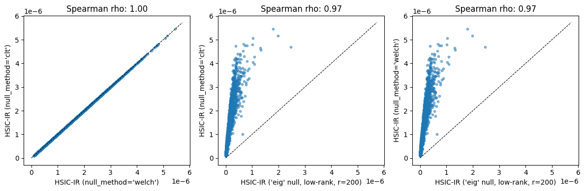
'welch' and 'clt' differ in their null distribution, with the former being a scaled chi-square distribution and the latter being a normal distribution. In practice, the p-values are highly concordant between the two except for extremely strong signals (near-zero p-values). On the other hand, 'eig' prioritizes low-frequency global patterns by design, and thus have more power detecting these patterns. The trade-off, however, is that it loses power entirely for high-frequency local patterns.

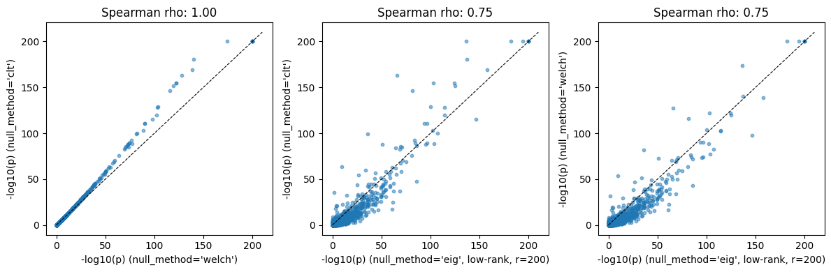
Biologically relevant spatial patterns are generally smooth (and global). In this brain dataset, the three methods yield concordant SVP rankings despite the power differences mentioned above.

for _pval in ['pvalue_eig', 'pvalue_welch', 'pvalue_clt']:
    merged[f'{_pval}_nl'] = -np.log10(merged[_pval].astype(float).clip(lower=1e-200))

rho_pval_eig_clt, _ = spearmanr(merged["pvalue_eig_nl"], merged["pvalue_clt_nl"])
rho_pval_welch_clt, _ = spearmanr(merged["pvalue_welch_nl"], merged["pvalue_clt_nl"])
rho_pval_eig_welch, _ = spearmanr(merged["pvalue_eig_nl"], merged["pvalue_welch_nl"])

def _format_axis_title(str):
    if str == "pvalue_eig_nl":
        return "-log10(p) (null_method='eig', low-rank, r=200)"
    elif str == "pvalue_welch_nl":
        return "-log10(p) (null_method='welch')"
    elif str == "pvalue_clt_nl":
        return "-log10(p) (null_method='clt')"

fig, axes = plt.subplots(1, 3, figsize=(12, 4))
for ax, (x, y, rho) in zip(axes,
    [("pvalue_welch_nl", "pvalue_clt_nl", rho_pval_welch_clt), 
     ("pvalue_eig_nl", "pvalue_clt_nl", rho_pval_eig_clt), 
     ("pvalue_eig_nl", "pvalue_welch_nl", rho_pval_eig_welch)]
):
    ax.scatter(merged[x], merged[y], alpha=0.5, s=10)
    lim = max(ax.get_xlim()[1], ax.get_ylim()[1])
    ax.plot([0, lim], [0, lim], "k--", lw=0.8, label="y = x")
    ax.set_xlabel(_format_axis_title(x))
    ax.set_ylabel(_format_axis_title(y))
    ax.set_title(f"Spearman rho: {rho:.2f}")

plt.tight_layout()
plt.show()

# Concordance at FDR < 1%
both_sig = set(sv_eig_sig["gene"]) & set(sv_clt_sig["gene"])
only_eig = set(sv_eig_sig["gene"]) - set(sv_clt_sig["gene"])
only_trace = set(sv_clt_sig["gene"]) - set(sv_eig_sig["gene"])
print(f"Concordant (both FDR<1%):  {len(both_sig)}")
print(f"Only eig significant:      {len(only_eig)}")
print(f"Only trace significant:    {len(only_trace)}")

Concordant (both FDR<1%):  755
Only eig significant:      704
Only trace significant:    65

For the significant SVP calls from only one method, the p-value is typically near the borderline, suggesting that this is mostly a power issue.

merged[
    ['gene', 'pvalue_eig', 'pvalue_clt', 'pvalue_welch']
].query('gene in @only_eig').sort_values('pvalue_eig', ascending=False).head(3)

	gene	pvalue_eig	pvalue_clt	pvalue_welch
2136	Pdgfa	0.004679	0.032410	0.033326
2801	Dnttip1	0.004655	0.250201	0.249278
2576	Grn	0.004603	0.018865	0.019671

merged[
    ['gene', 'pvalue_eig', 'pvalue_clt', 'pvalue_welch']
].query('gene in @only_trace').sort_values('pvalue_clt', ascending=False).head(3)

	gene	pvalue_eig	pvalue_clt	pvalue_welch
2198	Azi2	0.008135	0.002657	0.002957
2278	Kirrel	0.681066	0.002448	0.002734
2667	Gjb6	0.005113	0.002366	0.002645

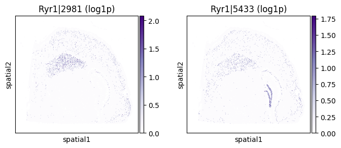
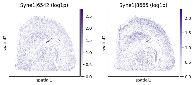
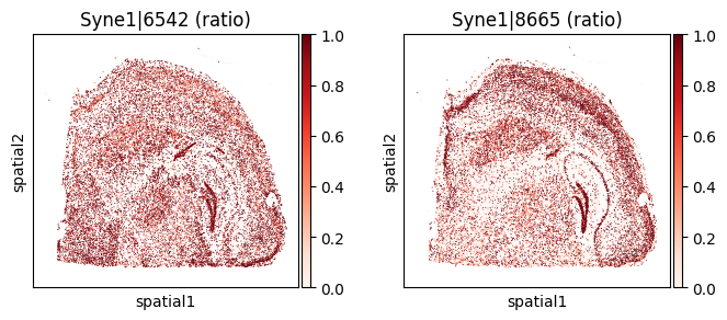
Visualize top SVP genes

top_genes = merged.sort_values('pvalue_eig').head(5)['gene'].tolist()
for _gene in top_genes[:3]:
    print(f"=== Plotting gene: {_gene} ===")
    _cw_to_plot = adata_codeword.var.query("gene_symbol == @_gene").index.tolist()
    _titles_log1p = [f"{_cw} (log1p)" for _cw in _cw_to_plot]
    _titles_ratio = [f"{_cw} (ratio)" for _cw in _cw_to_plot]
    with plt.rc_context({"figure.figsize": (3, 3)}):
        sc.pl.embedding(
            adata_codeword, basis='spatial', 
            color=_cw_to_plot, title=_titles_log1p,
            layer="log1p", cmap="Purples", vmin=0.0
        )
        sc.pl.embedding(
            adata_codeword, basis='spatial', 
            color=_cw_to_plot, title=_titles_ratio,
            layer="ratios_obs", cmap="Reds", vmin=0.0
        )

=== Plotting gene: Ryr1 ===

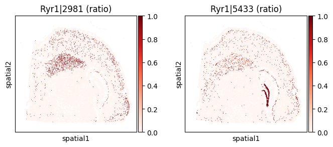
=== Plotting gene: Ckb ===

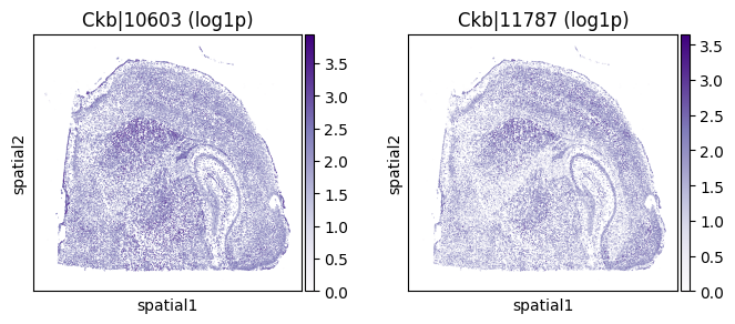
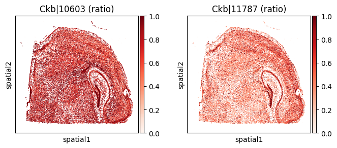
=== Plotting gene: Syne1 ===

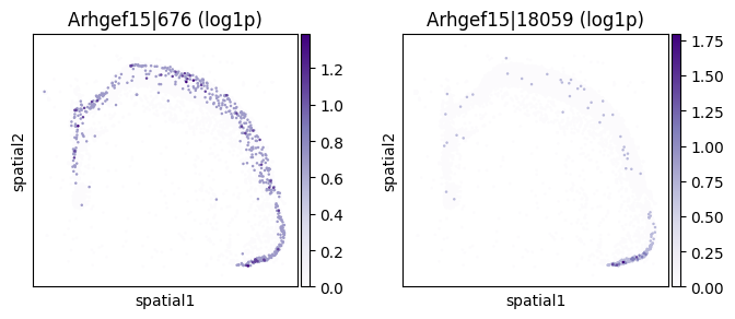
Within-cluster SVP genes

By subsetting to a single expression-based cluster, we can similarly identify spatially variable codeword usage within that cluster. Here we pick Cluster 2 (cortical neurons) as an example.

%%time
# Subset to cluster 2
adata_sub = adata_codeword[adata_codeword.obs['leiden'] == '2']

model_sv_sub = SplisosmNP(
    k_neighbors=4,
    rho=0.99,
    standardize_cov=True # will slow down .setup_data
)
model_sv_sub.setup_data(
    adata=adata_sub,
    spatial_key="spatial",
    layer="counts",
    group_iso_by=group_iso_by,
    gene_names=gene_name_col,
    min_counts=min_counts,
    min_bin_pct=min_bin_pct,
    filter_single_iso_genes=True,
    min_component_size=4, # remove disconnected tissue fragments with very few cells
)
model_sv_sub

/Users/jysumac/Projects/SPLISOSM/splisosm/hyptest_np.py:621: UserWarning: Removed 312 spot(s) belonging to graph components with fewer than 4 member(s). 9021 spot(s) remain.
  ) = prepare_inputs_from_anndata(

CPU times: user 1.11 s, sys: 341 ms, total: 1.45 s
Wall time: 1.17 s

=== SplisosmNP
- Number of genes: 2657
- Number of spots: 9021
- Number of covariates: 0
- Average isoforms per gene: 2.1
=== Model configurations
- Spatial kernel source: spatial_key='spatial' (component-filtered)
- k_neighbors: 4, rho: 0.99
- Standardize spatial covariance: True
=== Test results
- Spatial variability: N/A
- Differential usage: N/A

%%time
model_sv_sub.test_spatial_variability(
    method="hsic-ir",
    null_method="clt",
    ratio_transformation="none",
    nan_filling="mean",
    print_progress=True,
)
sv_sub = model_sv_sub.get_formatted_test_results("sv", with_gene_summary=True)
sv_sub.sort_values("pvalue_adj").head(5)

SV [hsic-ir]: 100%|██████████| 2657/2657 [00:01<00:00, 1731.19it/s]

CPU times: user 3 s, sys: 3.51 s, total: 6.51 s
Wall time: 2.41 s

	gene	statistic	pvalue	pvalue_adj	n_isos	perplexity	pct_bin_on	count_avg	count_std	major_ratio_avg
206	Arhgef15	0.000006	1.770860e-187	4.705175e-184	2	1.757146	0.077486	0.089569	0.334875	0.748762
2200	Ckb	0.000029	1.708663e-171	2.269958e-168	2	1.988247	0.941692	7.050770	5.190899	0.554233
1416	Rtn3	0.000023	1.041333e-84	9.222741e-82	2	1.915458	0.936149	6.920075	5.431430	0.645885
1565	Syne1	0.000036	3.838711e-73	2.549864e-70	2	1.872818	0.621993	1.305288	1.467576	0.679236
1863	Sncb	0.000012	1.052018e-50	5.590424e-48	2	1.822768	0.963086	13.934819	10.792033	0.711995

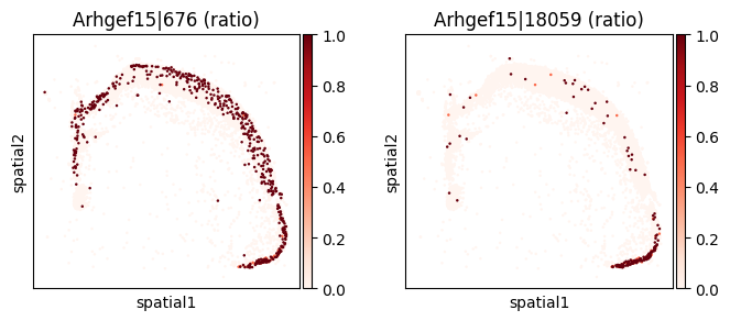
_gene = sv_sub.sort_values("pvalue_adj").iloc[0]["gene"]
print(f"=== Plotting gene: {_gene} ===")
_cw_to_plot = adata_codeword.var.query("gene_symbol == @_gene").index.tolist()
_titles_log1p = [f"{_cw} (log1p)" for _cw in _cw_to_plot]
_titles_ratio = [f"{_cw} (ratio)" for _cw in _cw_to_plot]
with plt.rc_context({"figure.figsize": (3, 3)}):
    sc.pl.embedding(
        adata_sub, basis='spatial', 
        color=_cw_to_plot, title=_titles_log1p,
        layer="log1p", cmap="Purples", vmin=0.0
    )
    sc.pl.embedding(
        adata_sub, basis='spatial', 
        color=_cw_to_plot, title=_titles_ratio,
        layer="ratios_obs", cmap="Reds", vmin=0.0
    )

=== Plotting gene: Arhgef15 ===

Differential codeword usage (DU) testing

Let’s focus our analysis on the set of significant SVP genes with spatially variable codeword usage.

# Keep only SVP genes for downstream DU testing
svp_gene_list = sv_clt.query("pvalue_adj < 0.01")["gene"].tolist()
svp_mask = adata_codeword.var["gene_symbol"].isin(svp_gene_list)
adata_svp = adata_codeword[:, svp_mask].copy()

print(f"Keeping {adata_svp.n_vars} codewords from {len(svp_gene_list)} SVP genes (FDR < 1% by trace test)")

Keeping 1777 codewords from 820 SVP genes (FDR < 1% by trace test)

Find cluster-specific SVP genes

Using the gene-expression-defined leiden clusters, we can run the differential usage test to find cluster-specific codeword usage patterns. Later, we will show how to run a similar analysis without cluster annotation.

%%time
# Model setup
model_clu = SplisosmNP()
model_clu.setup_data(
    adata=adata_svp,
    spatial_key="spatial",
    layer="counts",
    design_mtx="leiden", # one-hot encode leiden clusters as covariates
    group_iso_by=group_iso_by,
    gene_names=gene_name_col,
    min_counts=min_counts,
    min_bin_pct=min_bin_pct,
    filter_single_iso_genes=True,
    min_component_size=4, # remove disconnected tissue fragments with very few cells
    skip_spatial_kernel=True # DU test does not require spatial kernel, so we can skip to save time
)
model_clu

/Users/jysumac/Projects/SPLISOSM/splisosm/hyptest_np.py:621: UserWarning: Removed 893 spot(s) belonging to graph components with fewer than 4 member(s). 62280 spot(s) remain.
  ) = prepare_inputs_from_anndata(

CPU times: user 566 ms, sys: 206 ms, total: 773 ms
Wall time: 884 ms

=== SplisosmNP
- Number of genes: 820
- Number of spots: 62280
- Number of covariates: 17
- Average isoforms per gene: 2.2
=== Model configurations
- Spatial kernel source: identity (skip_spatial_kernel=True)
- k_neighbors: N/A, rho: 0.99
- Standardize spatial covariance: True
=== Test results
- Spatial variability: N/A
- Differential usage: N/A

Conditional differential usage test

By default, method="hsic-gp" will remove potential spatial confounding through Gaussian process regression (GPR), reducing false positives (spurious cluster association driven by chance).

%%time
# Conditional test
model_clu.test_differential_usage(
    method="hsic-gp",
    residualize='cov_only', # run GPR only for cluster one-hot
    # N approximation for faster GP fitting
    # increase n_inducing for better accuracy at the cost of speed
    gpr_configs={"covariate": {"n_inducing": 2000}},
    ratio_transformation="none",
    nan_filling="mean",
    print_progress=True,
)
clu_res_gp = model_clu.get_formatted_test_results("du")
clu_res_gp = clu_res_gp.rename(columns={
    "statistic": "stat_gp",
    "pvalue": "pvalue_gp"
})

Covariates:  35%|███▌      | 6/17 [00:14<00:25,  2.31s/it]/Users/jysumac/miniforge3/envs/splisosm_dev/lib/python3.12/site-packages/sklearn/gaussian_process/kernels.py:440: ConvergenceWarning: The optimal value found for dimension 0 of parameter k1__k1__constant_value is close to the specified lower bound 0.001. Decreasing the bound and calling fit again may find a better value.
  warnings.warn(
Covariates:  59%|█████▉    | 10/17 [00:24<00:17,  2.55s/it]/Users/jysumac/miniforge3/envs/splisosm_dev/lib/python3.12/site-packages/sklearn/gaussian_process/kernels.py:440: ConvergenceWarning: The optimal value found for dimension 0 of parameter k1__k1__constant_value is close to the specified lower bound 0.001. Decreasing the bound and calling fit again may find a better value.
  warnings.warn(
Covariates:  94%|█████████▍| 16/17 [00:40<00:02,  2.59s/it]/Users/jysumac/miniforge3/envs/splisosm_dev/lib/python3.12/site-packages/sklearn/gaussian_process/kernels.py:450: ConvergenceWarning: The optimal value found for dimension 0 of parameter k1__k1__constant_value is close to the specified upper bound 1000.0. Increasing the bound and calling fit again may find a better value.
  warnings.warn(
Covariates: 100%|██████████| 17/17 [00:42<00:00,  2.50s/it]
DU [hsic-gp]: 100%|██████████| 820/820 [00:09<00:00, 85.96it/s]

CPU times: user 59.7 s, sys: 34.2 s, total: 1min 33s
Wall time: 52.2 s

# Top 1 marker per cluster
clu_res_gp.groupby("covariate").apply(
    lambda df: df.nsmallest(1, "pvalue_gp"),
    include_groups=False
)

		gene	stat_gp	pvalue_gp	pvalue_adj
covariate
leiden_0	578	Ccn2	0.000057	0.0	0.0
leiden_1	103	Sptbn2	0.000632	0.0	0.0
leiden_10	146	Arrb2	0.000220	0.0	0.0
leiden_11	402	Epb41l3	0.000725	0.0	0.0
leiden_12	760	Slc2a1	0.000400	0.0	0.0
leiden_13	4926	Crb2	0.000031	0.0	0.0
leiden_14	116	Sptbn2	0.000422	0.0	0.0
leiden_15	11983	Isl1	0.000039	0.0	0.0
leiden_16	3994	Ryr1	0.000244	0.0	0.0
leiden_2	104	Sptbn2	0.000350	0.0	0.0
leiden_3	11733	Kit	0.000063	0.0	0.0
leiden_4	582	Ccn2	0.000045	0.0	0.0
leiden_5	940	Arhgef15	0.000197	0.0	0.0
leiden_6	11345	Vxn	0.000214	0.0	0.0
leiden_7	2744	Fbxo2	0.000324	0.0	0.0
leiden_8	3357	Ppp1r1b	0.000180	0.0	0.0
leiden_9	8475	Syne1	0.000658	0.0	0.0

Most SVP genes have at least one significant cluster association, suggesting that cell type distribution is a major driver of spatial patterns of isoform usage. Importantly, codeword usage and cluster identity are not one-to-one. An alternative hierarchical cell type/state annotation may be required to explain more nuanced spatial patterns.

_du_clu_sig = clu_res_gp.query('pvalue_adj < 0.05')
print(f"Cluster-specific DU genes (FDR < 5%): {len(_du_clu_sig['gene'].unique())} / {clu_res_gp['gene'].nunique()}")
print(f"Mean cluster associations per SVP gene: {_du_clu_sig.groupby('gene')['covariate'].nunique().mean():.2f}")

Cluster-specific DU genes (FDR < 5%): 816 / 820
Mean cluster associations per SVP gene: 7.96

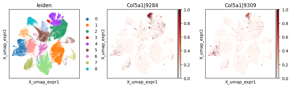
Visualize top cluster-specific codeword usage events

We can visualize top cluster-specific SVP genes on the UMAP computed from gene expression.

_clu = 'leiden_0'
_gene = clu_res_gp.query('covariate == @_clu').sort_values('pvalue_gp').iloc[0]['gene']
_cw_to_plot = adata_svp.var_names[adata_svp.var["gene_symbol"] == _gene].tolist()
print(f"Cluster-specific codeword usage for clu={_clu}, gene={_gene}")
with plt.rc_context({"figure.figsize": (3, 3)}):
    sc.pl.embedding(
        adata_svp, basis='X_umap_expr', 
        color=["leiden"] + _cw_to_plot, layer="ratios_obs", 
        cmap="Reds", vmin=0.0
    )

Cluster-specific codeword usage for clu=leiden_0, gene=Col5a1

And also in the physical space.

_clu = 'leiden_0'
_gene = clu_res_gp.query('covariate == @_clu').sort_values('pvalue_gp').iloc[0]['gene']
_cw_to_plot = adata_svp.var_names[adata_svp.var["gene_symbol"] == _gene].tolist()
print(f"Cluster-specific codeword usage for clu={_clu}, gene={_gene}")
with plt.rc_context({"figure.figsize": (3, 3)}):
    sc.pl.embedding(
        adata_svp, basis='spatial', 
        color=["leiden"] + _cw_to_plot, layer="ratios_obs", 
        cmap="Reds", vmin=0.0
    )

Cluster-specific codeword usage for clu=leiden_0, gene=Col5a1

Comparison with unconditional differential usage tests

We can also run unconditional tests, including the conventional two-sample T-test (method="t-fisher") and the unconditional HSIC test (method="hsic"). These tests are faster but may generate false positives due to spatial confounding.

%%time
# HSIC (multivariate RV coefficient)
model_clu.test_differential_usage(
    method="hsic",
    ratio_transformation="none",
    nan_filling="mean",
    print_progress=True,
)
clu_res_hsic = model_clu.get_formatted_test_results("du")
clu_res_hsic = clu_res_hsic.rename(columns={
    "statistic": "stat_hsic",
    "pvalue": "pvalue_hsic"
})

DU [hsic]: 100%|██████████| 820/820 [00:09<00:00, 84.59it/s]

CPU times: user 16.5 s, sys: 27.9 s, total: 44.4 s
Wall time: 9.86 s

%%time
# T-test (per-isoform pvalues combined by Fishers method)
model_clu.test_differential_usage(
    method="t-fisher",
    ratio_transformation="none",
    nan_filling="mean",
    print_progress=True,
)
clu_res_t = model_clu.get_formatted_test_results("du")
clu_res_t = clu_res_t.rename(columns={
    "statistic": "stat_t",
    "pvalue": "pvalue_t"
})

DU [t-fisher]: 100%|██████████| 820/820 [00:15<00:00, 52.10it/s]

CPU times: user 1min 28s, sys: 11.2 s, total: 1min 40s
Wall time: 16 s

def _neg_log10(p, floor=1e-300):
    return -np.log10(np.clip(p, floor, 1.0))

merge_cols = ["gene", "covariate"]

clu_all = (
    clu_res_gp[merge_cols + ["pvalue_gp"]]
    .merge(clu_res_hsic[merge_cols + ["pvalue_hsic"]], on=merge_cols, how="inner")
    .merge(clu_res_t[merge_cols + ["pvalue_t"]], on=merge_cols, how="inner")
)

# Spearman correlations between DU methods
rho_gp_hsic, _  = spearmanr(clu_all["pvalue_gp"],    clu_all["pvalue_hsic"])
rho_gp_t, _ = spearmanr(clu_all["pvalue_gp"],    clu_all["pvalue_t"])
rho_hsic_t, _  = spearmanr(clu_all["pvalue_hsic"],    clu_all["pvalue_t"])

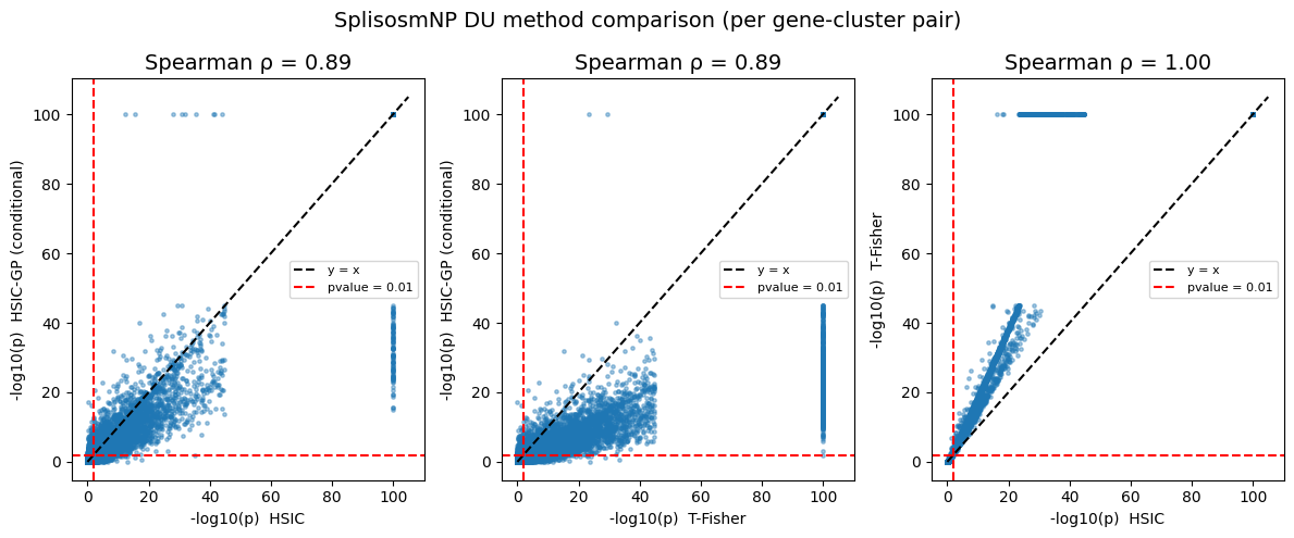
print(f"Spearman ρ(HSIC-GP vs HSIC) = {rho_gp_hsic:.3f}")
print(f"Spearman ρ(HSIC-GP vs T-Fisher) = {rho_gp_t:.3f}")
print(f"Spearman ρ(HSIC vs T-Fisher) = {rho_hsic_t:.3f}")

Spearman ρ(HSIC-GP vs HSIC) = 0.890
Spearman ρ(HSIC-GP vs T-Fisher) = 0.889
Spearman ρ(HSIC vs T-Fisher) = 0.998

The results between HSIC and T-test are highly similar (the test statistics are indeed equivalent, and the difference in p-values is mainly due to different choice of null distribution). On the other hand, the conditional HSIC-GP test is more conservative and yields shrinking p-values, as expected.

pairs_clu = [
    ("pvalue_hsic",    "pvalue_gp",
     "HSIC", "HSIC-GP (conditional)",  rho_gp_hsic),
    ("pvalue_t",       "pvalue_gp",
     "T-Fisher", "HSIC-GP (conditional)",  rho_gp_t),
    ("pvalue_hsic",    "pvalue_t",
     "HSIC", "T-Fisher",  rho_hsic_t),
]

fig, axes = plt.subplots(1, 3, figsize=(12, 5))
for ax, (cx, cy, lx, ly, rho) in zip(axes, pairs_clu):
    x = _neg_log10(clu_all[cx].astype(float).values, floor=1e-100)
    y = _neg_log10(clu_all[cy].astype(float).values, floor=1e-100)
    ax.scatter(x, y, s=6, alpha=0.4, rasterized=True)
    lim = max(x.max(), y.max()) * 1.05
    ax.plot([0, lim], [0, lim], "k--", label="y = x")
    ax.axhline(_neg_log10(0.01), color="red", linestyle="--", label="pvalue = 0.01")
    ax.axvline(_neg_log10(0.01), color="red", linestyle="--")
    ax.set_xlabel(f"-log10(p)  {lx}", fontsize=10)
    ax.set_ylabel(f"-log10(p)  {ly}", fontsize=10)
    ax.set_title(f"Spearman ρ = {rho:.2f}", fontsize=14)
    ax.legend(fontsize=8)

fig.suptitle("SplisosmNP DU method comparison (per gene-cluster pair)", fontsize=14)
fig.tight_layout()
plt.show()

Find potential RBP regulators of SVP genes

Next, we can test for associations between codeword usage of SVP genes and RBP expression to find potential regulators of the observed patterns.

# Build RBP covariate matrix
# A subset of splicing-regulatory RBPs; adapt to the genes in your panel.
rbp_genes = {
    'Ago2', 'Celf', 'Celf1', 'Celf2', 'Celf3', 'Celf4', 'Celf5', 'Celf6', 
    'Elavl1', 'Elavl2', 'Elavl3', 'Elavl4', 'Fus', 
    'Mbnl1', 'Mbnl2', 'Mbnl3', 'Msi1', 'Msi2', 'Nova1', 'Nova2', 
    'Pabpc1', 'Pabpc1l', 'Pabpc2', 'Pabpc4', 'Pabpc5', 'Pabpc6', 'Pabpn1', 
    'Pcbp1', 'Pcbp2', 'Pcbp3', 'Pcbp4', 'Ptbp1', 'Ptbp2', 
    'Qk', 'Rbfox1', 'Rbfox2', 'Rbfox3', 
    'Srsf1', 'Srsf10', 'Srsf12', 'Srsf2', 'Srsf3', 'Srsf4',
    'Srsf5', 'Srsf6', 'Srsf7', 'Srsf9',
}

# Find overlapping genes
rbp_used = [
    rbp for rbp in rbp_genes 
    if rbp in adata_gene.var_names]
print(f"RBP genes in panel: {len(rbp_used)} / {len(rbp_genes)}")
if len(rbp_used) == 0:
    raise RuntimeError(
        "No RBP genes found in the panel. "
        "Check gene name format or extend the rbp_genes list."
    )

# Compute RBP covariate matrix
design_mtx = adata_gene[:, rbp_used].layers["log1p"].copy()
covariate_names = rbp_used
print(f"Design matrix: {design_mtx.shape}  ({len(rbp_used)} RBP covariates)")

RBP genes in panel: 17 / 47
Design matrix: (63173, 17)  (17 RBP covariates)

%%time
# Model setup for DU testing
model_rbp = SplisosmNP()
model_rbp.setup_data(
    adata=adata_svp,
    spatial_key="spatial",
    layer="counts",
    design_mtx=design_mtx,
    covariate_names=covariate_names,
    group_iso_by=group_iso_by,
    gene_names=gene_name_col,
    min_counts=min_counts,
    min_bin_pct=min_bin_pct,
    filter_single_iso_genes=True,
    min_component_size=4, # remove disconnected tissue fragments with very few cells
    skip_spatial_kernel=True # DU test does not require spatial kernel, so we can skip to save time
)
model_rbp

/Users/jysumac/Projects/SPLISOSM/splisosm/hyptest_np.py:621: UserWarning: Removed 893 spot(s) belonging to graph components with fewer than 4 member(s). 62280 spot(s) remain.
  ) = prepare_inputs_from_anndata(

CPU times: user 453 ms, sys: 177 ms, total: 630 ms
Wall time: 651 ms

=== SplisosmNP
- Number of genes: 820
- Number of spots: 62280
- Number of covariates: 17
- Average isoforms per gene: 2.2
=== Model configurations
- Spatial kernel source: identity (skip_spatial_kernel=True)
- k_neighbors: N/A, rho: 0.99
- Standardize spatial covariance: True
=== Test results
- Spatial variability: N/A
- Differential usage: N/A

%%time
model_rbp.test_differential_usage(
    method="hsic-gp",
    residualize='cov_only', # run GPR only for RBP covariates
    # N approximation for faster GP fitting
    # increase n_inducing for better accuracy at the cost of speed
    gpr_configs={"covariate": {"n_inducing": 2000}},
    ratio_transformation="none",
    nan_filling="mean",
    print_progress=True,
)
du_res = model_rbp.get_formatted_test_results("du")

Covariates:  59%|█████▉    | 10/17 [00:26<00:18,  2.71s/it]/Users/jysumac/miniforge3/envs/splisosm_dev/lib/python3.12/site-packages/sklearn/gaussian_process/kernels.py:440: ConvergenceWarning: The optimal value found for dimension 0 of parameter k1__k1__constant_value is close to the specified lower bound 0.001. Decreasing the bound and calling fit again may find a better value.
  warnings.warn(
Covariates:  71%|███████   | 12/17 [00:32<00:13,  2.78s/it]/Users/jysumac/miniforge3/envs/splisosm_dev/lib/python3.12/site-packages/sklearn/gaussian_process/kernels.py:440: ConvergenceWarning: The optimal value found for dimension 0 of parameter k1__k1__constant_value is close to the specified lower bound 0.001. Decreasing the bound and calling fit again may find a better value.
  warnings.warn(
Covariates:  88%|████████▊ | 15/17 [00:40<00:05,  2.80s/it]/Users/jysumac/miniforge3/envs/splisosm_dev/lib/python3.12/site-packages/sklearn/gaussian_process/kernels.py:440: ConvergenceWarning: The optimal value found for dimension 0 of parameter k1__k1__constant_value is close to the specified lower bound 0.001. Decreasing the bound and calling fit again may find a better value.
  warnings.warn(
Covariates: 100%|██████████| 17/17 [00:46<00:00,  2.71s/it]
DU [hsic-gp]: 100%|██████████| 820/820 [00:09<00:00, 85.76it/s]

CPU times: user 1min 2s, sys: 37.7 s, total: 1min 39s
Wall time: 55.8 s

du_sig = du_res[du_res["pvalue_adj"] < 0.05].sort_values("pvalue_adj")
print(f"Significant gene–RBP associations (FDR < 5%): {len(du_sig)}")
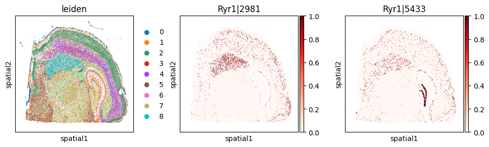
du_sig.query("gene == 'Ryr1'").head(5)

Significant gene–RBP associations (FDR < 5%): 5716

	gene	covariate	statistic	pvalue	pvalue_adj
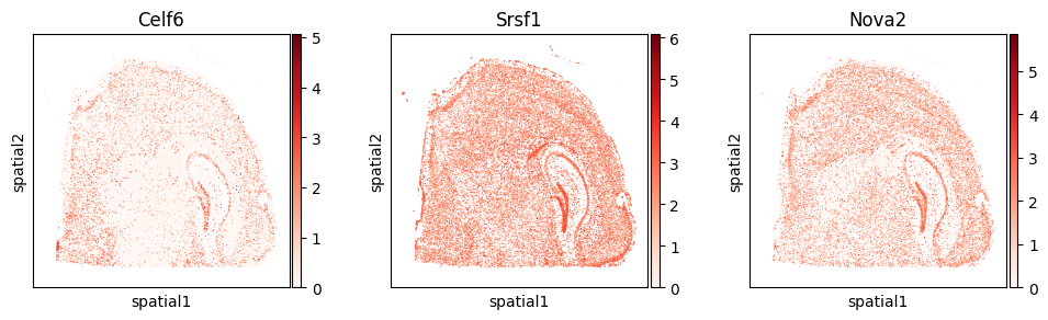
3985	Ryr1	Celf6	0.000014	1.029617e-09	1.623627e-08
3988	Ryr1	Srsf1	0.000008	3.302417e-06	6.150645e-05
3980	Ryr1	Nova2	0.000003	2.537556e-03	5.176109e-03

_cw_to_plot = adata_svp.var.query("gene_symbol == 'Ryr1'").index.tolist()
with plt.rc_context({"figure.figsize": (3, 3)}):
    sc.pl.embedding(
        adata_svp, basis='spatial', 
        color=["leiden"] + _cw_to_plot, layer="ratios_obs", 
        cmap="Reds", vmin=0.0
    )

with plt.rc_context({"figure.figsize": (3, 3)}):
    sc.pl.embedding(
        adata_gene, basis='spatial', 
        color=["Celf6", "Srsf1", "Nova2"], layer="log1p", 
        cmap="Reds", vmin=0.0
    )

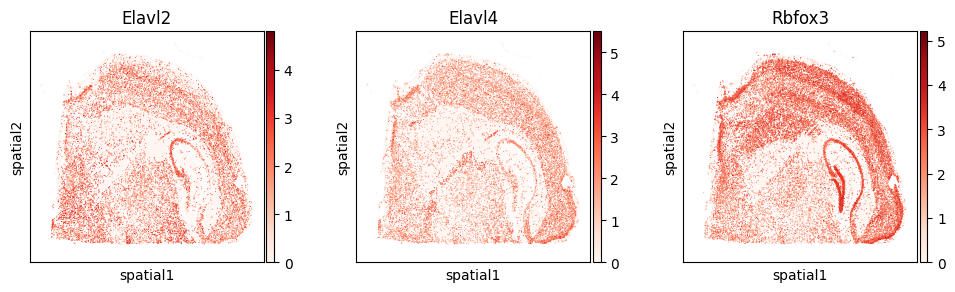
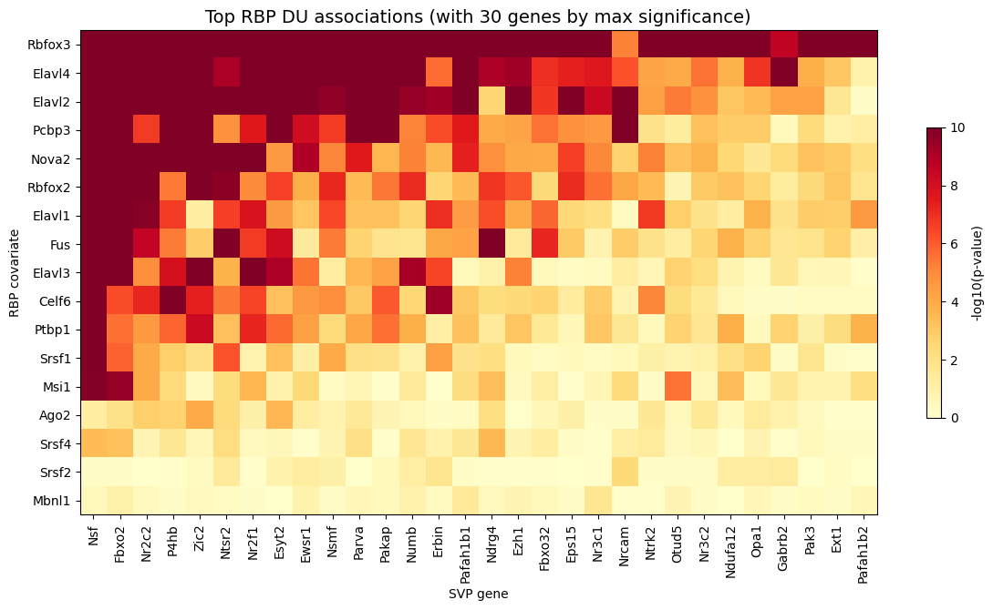
The most significant splicing factors in our analysis include Elavl2, Elavl4, and Rbfox3.

with plt.rc_context({"figure.figsize": (3, 3)}):
    sc.pl.embedding(
        adata_gene, basis='spatial', 
        color=["Elavl2", "Elavl4", "Rbfox3"], layer="log1p", 
        cmap="Reds", vmin=0.0
    )

# Pivot to gene × RBP matrix of -log10(adjusted p-values)
pivot = du_res.pivot_table(
    index="gene", columns="covariate", values="pvalue", fill_value=1.0
)
log_p = -np.log10(pivot.clip(lower=1e-10))

# Select top 30 genes by maximum significance across all covariates
top_genes_du = log_p.max(axis=1).sort_values(ascending=False).head(30).index
log_p_top = log_p.loc[top_genes_du]

# Rank rows and columns by mean significance
log_p_transposed = log_p_top.T
rbp_order = log_p_transposed.mean(axis=1).sort_values(ascending=False).index
gene_order = log_p_transposed.mean(axis=0).sort_values(ascending=False).index
log_p_final = log_p_transposed.loc[rbp_order, gene_order]

# Plottting the heatmap
fig, ax = plt.subplots(figsize=(12, max(6, len(rbp_order) * 0.4)))
im = ax.imshow(log_p_final.values, aspect="auto", cmap="YlOrRd", vmin=0)
ax.set_xticks(range(len(log_p_final.columns)))
ax.set_xticklabels(log_p_final.columns, rotation=90, ha="center", fontsize=10) 
ax.set_yticks(range(len(log_p_final.index)))
ax.set_yticklabels(log_p_final.index, fontsize=10)

# Update axis labels
ax.set_xlabel("SVP gene")
ax.set_ylabel("RBP covariate")
ax.set_title(
    "Top RBP DU associations (with 30 genes by max significance)",
    fontsize=14
)

plt.colorbar(im, ax=ax, label="-log10(p-value)", shrink=0.6)
plt.tight_layout()
plt.show()

Variability testing on a custom graph

Instead of using physical spatial coordinates, we can leverage the expression-based k-NN graph from sc.pp.neighbors() to detect codeword usage variability across the cell population. This approach identifies genes whose isoform usage varies across “transcriptomic neighborhoods” and continuous cell states. Conceptually, it is similar to the Moran’s I-based Hostpot analysis for gene variability.

%%time
# adata_codeword.obsp['expr_knn'] = adata_gene[adata_codeword.obs_names].obsp['connectivities'].copy()

model_expr_sv = SplisosmNP(
    rho=0.99,
    standardize_cov=False, # faster
)
model_expr_sv.setup_data(
    adata=adata_codeword,
    adj_key='expr_knn',  # use expression graph instead of spatial coordinates
    layer='counts',
    group_iso_by=group_iso_by,
    gene_names=gene_name_col,
    min_counts=min_counts,
    min_bin_pct=min_bin_pct,
    filter_single_iso_genes=True,
    min_component_size=4, # same filtering but now based on expression graph connectivity
)
model_expr_sv

CPU times: user 1.01 s, sys: 667 ms, total: 1.68 s
Wall time: 1.94 s

=== SplisosmNP
- Number of genes: 3059
- Number of spots: 63173
- Number of covariates: 0
- Average isoforms per gene: 2.1
=== Model configurations
- Spatial kernel source: adj_key='expr_knn'
- k_neighbors: N/A, rho: 0.99
- Standardize spatial covariance: False
=== Test results
- Spatial variability: N/A
- Differential usage: N/A

%%time
model_expr_sv.test_spatial_variability(
    method='hsic-ir',
    null_method='clt',  # fast; no eigendecomposition needed
    print_progress=True,
)
sv_expr = model_expr_sv.get_formatted_test_results('sv', with_gene_summary=True)

SV [hsic-ir]: 100%|██████████| 3059/3059 [05:22<00:00,  9.49it/s]

CPU times: user 45min 3s, sys: 45.3 s, total: 45min 48s
Wall time: 7min 30s

sv_expr_sig = sv_expr.query('pvalue_adj < 0.01')
print(f"Expression-SVP genes (FDR < 1%): {len(sv_expr_sig)} / {len(sv_expr)}")
sv_expr.sort_values('pvalue').head(5)

Expression-SVP genes (FDR < 1%): 2598 / 3059

	gene	statistic	pvalue	pvalue_adj	n_isos	perplexity	pct_bin_on	count_avg	count_std	major_ratio_avg
1897	Dlgap4	0.000005	0.0	0.0	3	2.945969	0.430184	0.767321	1.181466	0.397203
2327	Pafah1b1	0.000005	0.0	0.0	2	1.963350	0.529467	0.912953	1.146167	0.595866
2328	Camk2d	0.000001	0.0	0.0	2	1.524235	0.286277	0.532458	1.130050	0.850700
513	Mapk10	0.000004	0.0	0.0	2	1.968198	0.455052	0.984962	1.485261	0.589284
242	Arhgef15	0.000003	0.0	0.0	2	1.970105	0.083564	0.099394	0.357920	0.586558

Compare expression-SVP genes with spatial-SVP genes

We can compare the expression-SVP gene set with the spatial-SVP genes identified earlier.

expr_svp_genes = set(sv_expr.query('pvalue_adj < 0.01')['gene'])
spatial_svp_genes = set(sv_clt.query('pvalue_adj < 0.01')['gene'])

print(f"Spatial SVP genes (physical coords):  {len(spatial_svp_genes)}")
print(f"Expression SVP genes (expr k-NN):     {len(expr_svp_genes)}")
print(f"Spatial SVP ∩ Expression SVP:          {len(spatial_svp_genes & expr_svp_genes)}")

Spatial SVP genes (physical coords):  820
Expression SVP genes (expr k-NN):     2598
Spatial SVP ∩ Expression SVP:          808

merged = (
    sv_clt[["gene", "statistic", "pvalue"]].rename(columns={
        "statistic": "stat_sp",
        "pvalue": "pvalue_sp"
    }).merge(
        sv_expr[["gene", "statistic", "pvalue"]].rename(columns={
            "statistic": "stat_expr", 
            "pvalue": "pvalue_expr"
        }),
        on="gene",
    )
)
rho_stat, _ = spearmanr(merged["stat_sp"], merged["stat_expr"])
rho_pval, _ = spearmanr(
    -np.log10(merged["pvalue_sp"].astype(float).clip(lower=1e-300)), 
    -np.log10(merged["pvalue_expr"].astype(float).clip(lower=1e-300))
)

fig, ax = plt.subplots(figsize=(5, 5))
ax.scatter(
    -np.log10(merged["pvalue_sp"].astype(float).clip(lower=1e-300)),
    -np.log10(merged["pvalue_expr"].astype(float).clip(lower=1e-300)),
    alpha=0.4, s=10, c="steelblue", rasterized=True,
)
lim = max(ax.get_xlim()[1], ax.get_ylim()[1])
ax.plot([0, lim], [0, lim], "k--", lw=0.8, label="y = x")
ax.set_xlabel("-log10(p) (spatial graph)")
ax.set_ylabel("-log10(p) (expression graph)")
ax.set_title(f"P-value (Spearman ρ={rho_pval:.3f})")
ax.legend()
plt.tight_layout()
plt.show()

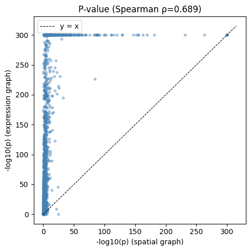
Most spatially variably processed genes also show variability across the expression-based cell embedding space, with few exceptions:

merged.query('gene in @spatial_svp_genes').sort_values('pvalue_expr', ascending=False).head(5)

	gene	stat_sp	pvalue_sp	stat_expr	pvalue_expr
65	Spink8	1.572542e-07	8.064405e-26	1.492586e-07	0.817782
2645	Grm8	1.121168e-06	1.067065e-04	1.193935e-06	0.286051
1383	Pou3f2	8.047140e-07	3.496205e-06	8.358410e-07	0.249884
1151	Rnf219	5.967543e-07	2.296819e-03	6.383463e-07	0.164888
2667	Cd83	4.825617e-07	1.139044e-03	5.138477e-07	0.144273

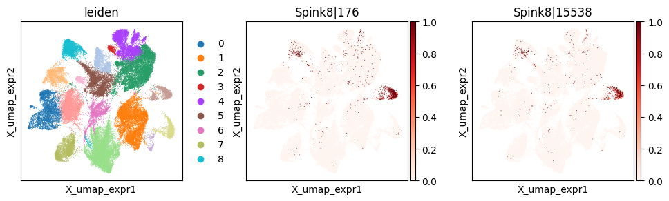
_gene = 'Spink8'
print(f"Codeword usage for gene={_gene} (SVP by spatial graph, not by expression graph)")

_cw_to_plot = adata_svp.var_names[adata_svp.var["gene_symbol"] == _gene].tolist()
with plt.rc_context({"figure.figsize": (3, 3)}):
    sc.pl.embedding(
        adata_svp, basis='X_umap_expr', 
        color=["leiden"] + _cw_to_plot, layer="ratios_obs", 
        cmap="Reds", vmin=0.0
    )
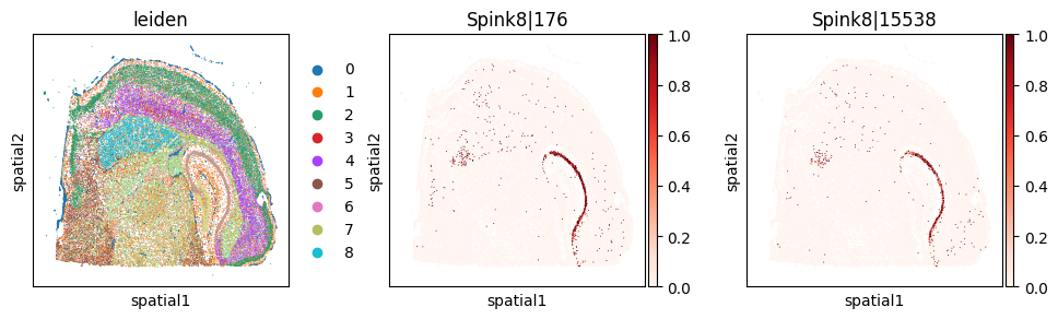
with plt.rc_context({"figure.figsize": (3, 3)}):
    sc.pl.embedding(
        adata_svp, basis='spatial', 
        color=["leiden"] + _cw_to_plot, layer="ratios_obs", 
        cmap="Reds", vmin=0.0
    )

Codeword usage for gene=Spink8 (SVP by spatial graph, not by expression graph)

merged.query('gene not in @spatial_svp_genes').sort_values('pvalue_expr').head(5)

	gene	stat_sp	pvalue_sp	stat_expr	pvalue_expr
2748	Tox	2.630988e-07	0.125585	3.745561e-07	0.0
2683	Tmem43	2.658433e-07	0.006387	3.731942e-07	0.0
1384	Mafb	4.629190e-07	0.108365	8.195273e-07	0.0
1950	Erbb4	7.551144e-07	0.203368	1.087955e-06	0.0
602	Hspa5	2.931829e-06	0.012102	4.644539e-06	0.0

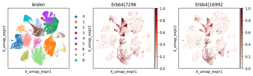
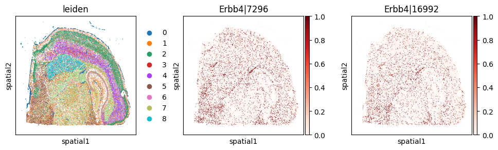
_gene = 'Erbb4'
print(f"Codeword usage for gene={_gene} (SVP by expression graph, not by spatial graph)")

_cw_to_plot = adata_codeword.var_names[adata_codeword.var["gene_symbol"] == _gene].tolist()
with plt.rc_context({"figure.figsize": (3, 3)}):
    sc.pl.embedding(
        adata_codeword, basis='X_umap_expr', 
        color=["leiden"] + _cw_to_plot, layer="ratios_obs", 
        cmap="Reds", vmin=0.0
    )
with plt.rc_context({"figure.figsize": (3, 3)}):
    sc.pl.embedding(
        adata_codeword, basis='spatial', 
        color=["leiden"] + _cw_to_plot, layer="ratios_obs", 
        cmap="Reds", vmin=0.0
    )

Codeword usage for gene=Erbb4 (SVP by expression graph, not by spatial graph)

Summary

• SplisosmNP’s SV tests can detect expression and codeword usage variability across both physical space and latent expression space.

• Different null_method choices ('eig', 'welch', 'clt') produce highly concordant rankings. Both moment matching and low-rank approximation scale well with increasing dataset size.

• The GP-detrended DU test (hsic-gp) controls false positives from spatial autocorrelation more rigorously than the unconditional test (hsic and T-tests).

For reproducibility

import sys
from datetime import date
import splisosm

print('Last updated:', date.today())
print('Python:', sys.version.split()[0])
print('splisosm:', getattr(splisosm, '__version__', 'unknown'))

Last updated: 2026-04-20
Python: 3.12.13
splisosm: 1.1.1