Visium HD FFPE (probe) Part I

This notebook is the first of two tutorials where we apply SPLISOSM to a probe-based Visium HD FFPE dataset of adult mouse brain. It covers the following steps:

1. Load probe-level quantification from Space Ranger outputs.

2. Run FFT-accelerated spatial variability tests with SplisosmFFT.

3. Check sensitivity to kernel hyperparameters.

4. Compare SV test results across spatial resolutions.

5. Compare SplisosmFFT and SplisosmNP results.

Next step: Visium HD FFPE (probe) Part II for differential usage analysis to find potential RNA-binding protein (RBP) regulators of genes with spatially variable isoform/peak/exon/junction usage.

The workflow is compatible with other ST platforms. See guidance on data preparation and the tutorial gallery for more examples.

Estimated runtime: ~10 min.

Preliminary notes

For FFPE samples, Visium HD uses pre-designed probes targeting specific transcript regions (e.g., exons, junctions) for sequencing and quantification. After running the Space Ranger count pipeline (v4.0+), a raw_probe_bc_matrix.h5 file of barcode-by-probe UMI count matrix is provided at 2um resolution, see 10x official documentation on output structures. We will load this matrix as well as gene-expression matrices as a SpatialData object and run SPLISOSM’s spatial variability (SV) tests.

The SPLISOSM package provides two implementations of the same sets of HSIC-based dependency tests:

• SplisosmFFT utilizes Fast Fourier Transform (FFT) to scale full-rank spatial kernels to dataset with millions of spots. It is faster and more accurate, but requires data on a regular grid (e.g., Visium HD bins).

• SplisosmNP uses low-rank kernel approximation to avoid quadratic memory scaling. It sacrifices power on high-frequency spatial patterns, but is compatible with any geometries such as cell-segmented data.

For technical details, see the Methods page and our associated preprint.

Imports

from __future__ import annotations

from itertools import combinations
from pathlib import Path
import warnings

import annsel as an
import numpy as np
import pandas as pd
import matplotlib.pyplot as plt
from scipy.stats import spearmanr

import spatialdata as sd
import spatialdata_plot
from spatialdata import rasterize_bins

from splisosm import SplisosmFFT, SplisosmNP
from splisosm.utils import counts_to_ratios
from splisosm.io import load_visiumhd_probe

warnings.filterwarnings("ignore", category=FutureWarning)
plt.rcParams["figure.dpi"] = 120
plt.rcParams["figure.figsize"] = (6, 4)

Configure paths and core parameters

# Required: Space Ranger `outs` directory for Visium HD
visium_hd_outs = Path("/path/to/visium_hd_ffpe/outs")

# Optional cache path for faster reruns
sdata_zarr = visium_hd_outs / "sdata_probe.filtered.zarr"

# Spatial resolutions (µm) to materialize in SpatialData
bin_sizes = [2, 8, 16]

# Dataset and table identifiers (16µm binning used throughout)
dataset_id = "Visium_HD_Mouse_Brain"
test_table = "square_016um"
test_bins_element = f"{dataset_id}_square_016um"

# Probe annotation column names
group_iso_by = "gene_ids"
candidate_gene_name_cols = ["gene_name", "gene_symbol", "gene_names"]

# Probe QC filters
min_counts = 10
min_bin_pct = 0.01

Load probe-level SpatialData

To run the analysis, please download the Space Ranger outs directory for the Visium HD adult mouse brain FFPE dataset from 10x Genomics (Visium Mouse Transcriptome Probe Set v2.1).

We use splisosm.io.load_visiumhd_probe to load data as a SpatialData object. The function wraps spatialdata-io.visium_hd. Setting filtered_counts_file=True keeps only barcodes that pass Space Ranger’s filtering (i.e., non-background bins retained in filtered_feature_bc_matrix).

%%time
if sdata_zarr.exists():
    print("Loading cached SpatialData...")
    sdata = sd.read_zarr(sdata_zarr)
else:
    print("Building probe-level SpatialData from Space Ranger outputs...")
    sdata = load_visiumhd_probe(
        path=visium_hd_outs,
        bin_sizes=bin_sizes,
        filtered_counts_file=True,
        load_all_images=False,
        var_names_make_unique=True,
        counts_layer_name="counts",
    )
    # Optional: cache for future runs
    # sdata.write(sdata_zarr)

sdata

Loading cached SpatialData...
CPU times: user 7.95 s, sys: 1.41 s, total: 9.36 s
Wall time: 5.41 s

SpatialData object, with associated Zarr store: /Users/jysumac/Projects/SPLISOSM_paper/data/visiumhd_ffpe_mouse_cbs/sdata_probe.filtered.zarr
├── Images
│     ├── 'Visium_HD_Mouse_Brain_full_image': DataTree[cyx] (3, 23947, 18872), (3, 11973, 9436), (3, 5986, 4718), (3, 2993, 2359), (3, 1496, 1179)
│     ├── 'Visium_HD_Mouse_Brain_hires_image': DataArray[cyx] (3, 6000, 4729)
│     └── 'Visium_HD_Mouse_Brain_lowres_image': DataArray[cyx] (3, 600, 473)
├── Shapes
│     ├── 'Visium_HD_Mouse_Brain_cell_segmentations': GeoDataFrame shape: (40222, 2) (2D shapes)
│     ├── 'Visium_HD_Mouse_Brain_square_002um': GeoDataFrame shape: (6296688, 1) (2D shapes)
│     ├── 'Visium_HD_Mouse_Brain_square_008um': GeoDataFrame shape: (393543, 1) (2D shapes)
│     └── 'Visium_HD_Mouse_Brain_square_016um': GeoDataFrame shape: (98917, 1) (2D shapes)
└── Tables
      ├── 'cell_segmentations': AnnData (40222, 55538)
      ├── 'square_002um': AnnData (6296688, 55538)
      ├── 'square_008um': AnnData (393543, 55538)
      └── 'square_016um': AnnData (98917, 55538)
with coordinate systems:
    ▸ 'Visium_HD_Mouse_Brain', with elements:
        Visium_HD_Mouse_Brain_full_image (Images), Visium_HD_Mouse_Brain_hires_image (Images), Visium_HD_Mouse_Brain_lowres_image (Images), Visium_HD_Mouse_Brain_cell_segmentations (Shapes), Visium_HD_Mouse_Brain_square_002um (Shapes), Visium_HD_Mouse_Brain_square_008um (Shapes), Visium_HD_Mouse_Brain_square_016um (Shapes)
    ▸ 'Visium_HD_Mouse_Brain_downscaled_hires', with elements:
        Visium_HD_Mouse_Brain_hires_image (Images), Visium_HD_Mouse_Brain_cell_segmentations (Shapes), Visium_HD_Mouse_Brain_square_002um (Shapes), Visium_HD_Mouse_Brain_square_008um (Shapes), Visium_HD_Mouse_Brain_square_016um (Shapes)
    ▸ 'Visium_HD_Mouse_Brain_downscaled_lowres', with elements:
        Visium_HD_Mouse_Brain_lowres_image (Images), Visium_HD_Mouse_Brain_cell_segmentations (Shapes), Visium_HD_Mouse_Brain_square_002um (Shapes), Visium_HD_Mouse_Brain_square_008um (Shapes), Visium_HD_Mouse_Brain_square_016um (Shapes)

SPLISOSM can be run at any spatial resolution, but data become sparser at finer scales.

def summarize_table(adata):
    X = adata.layers["counts"] if "counts" in adata.layers else adata.X
    if hasattr(X, "nnz"):
        nnz = int(X.nnz)
        total = int(X.shape[0] * X.shape[1])
        density = nnz / total if total else np.nan
    else:
        arr = np.asarray(X)
        nnz = int(np.count_nonzero(arr))
        total = int(arr.size)
        density = nnz / total if total else np.nan
    return {
        "n_probes": int(adata.n_vars),
        "n_bins": int(adata.n_obs),
        "count_mtx_density": density,
    }

rows = []
for key in sorted(sdata.tables.keys()):
    if key.startswith("square_"):
        rows.append({"table": key, **summarize_table(sdata.tables[key])})

table_summary = pd.DataFrame(rows).sort_values("table")
table_summary

	table	n_probes	n_bins	count_mtx_density
0	square_002um	55538	6296688	0.000253
1	square_008um	55538	393543	0.003819
2	square_016um	55538	98917	0.013923

To balance sparsity and computation, we recommend 16µm or 8µm bins for initial analysis. Resolution comparison is shown at the end of this notebook.

# Optional: inspect available coordinate systems and image/shape keys
print("Tables:", sorted(sdata.tables.keys()))
print("Images:", sorted(getattr(sdata, "images", {}).keys()))
print("Shapes:", sorted(getattr(sdata, "shapes", {}).keys()))

# Quick guardrails before model setup
if test_table not in sdata.tables:
    raise ValueError(f"{test_table} is not available. Choose from: {sorted(sdata.tables.keys())}")

adata_test = sdata.tables[test_table]
if group_iso_by not in adata_test.var.columns:
    raise ValueError(f"{group_iso_by} not found in {test_table}.var columns")

gene_name_col = None
for col in candidate_gene_name_cols:
    if col in adata_test.var.columns:
        gene_name_col = col
        break

print(f"Using table={test_table}, bins={test_bins_element}")
print(f"Grouping column={group_iso_by}, display names={gene_name_col}")

Tables: ['cell_segmentations', 'square_002um', 'square_008um', 'square_016um']
Images: ['Visium_HD_Mouse_Brain_full_image', 'Visium_HD_Mouse_Brain_hires_image', 'Visium_HD_Mouse_Brain_lowres_image']
Shapes: ['Visium_HD_Mouse_Brain_cell_segmentations', 'Visium_HD_Mouse_Brain_square_002um', 'Visium_HD_Mouse_Brain_square_008um', 'Visium_HD_Mouse_Brain_square_016um']
Using table=square_016um, bins=Visium_HD_Mouse_Brain_square_016um
Grouping column=gene_ids, display names=gene_name

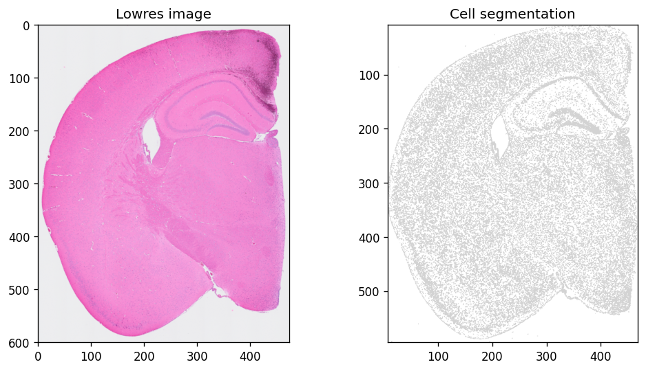
Use spatialdata-plot to visualize tissue morphology:

%%time
axes = plt.subplots(1, 2, figsize=(10, 5))[1].flatten()
sdata.pl.render_images(f"{dataset_id}_lowres_image").pl.show(
    coordinate_systems=f"{dataset_id}_downscaled_lowres",
    ax=axes[0], title="Lowres image"
)
sdata.pl.render_shapes(f"{dataset_id}_cell_segmentations").pl.show(
    coordinate_systems=f"{dataset_id}_downscaled_lowres",
    ax=axes[1], title="Cell segmentation"
)

CPU times: user 2.2 s, sys: 153 ms, total: 2.35 s
Wall time: 2.45 s

To visualize probe expression as an image, rasterize the spatial bins first:

%%time
for bin_size in ["016", "008", "002"]:
    # rasterize_bins() requires a compressed sparse column (csc) matrix
    sdata.tables[f"square_{bin_size}um"].X = sdata.tables[f"square_{bin_size}um"].X.tocsc()
    rasterized = rasterize_bins(
        sdata,
        f"{dataset_id}_square_{bin_size}um",
        f"square_{bin_size}um",
        "array_col",
        "array_row",
    )
    sdata[f"rasterized_{bin_size}um"] = rasterized

CPU times: user 4.56 s, sys: 834 ms, total: 5.39 s
Wall time: 5.49 s

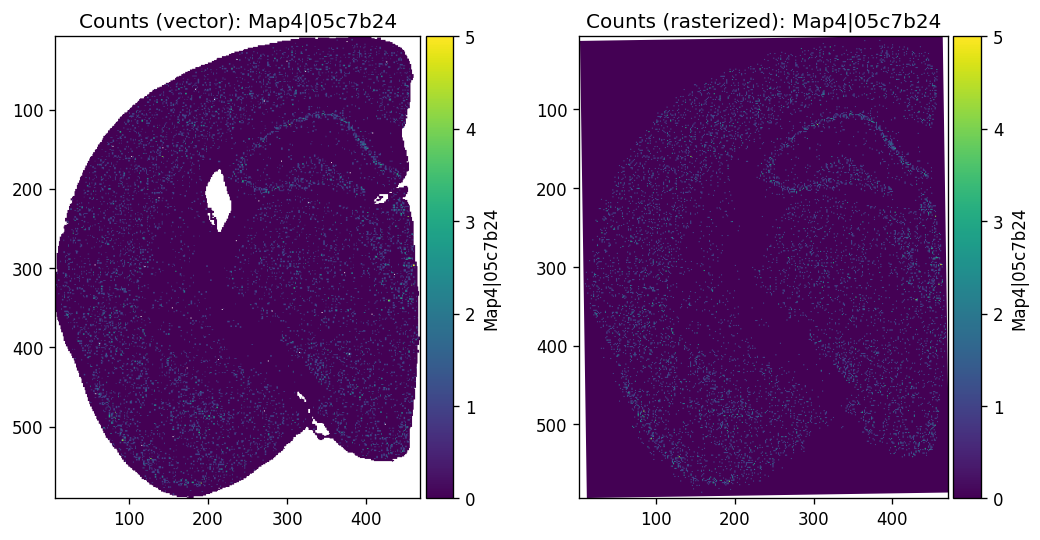
Then visualize a probe’s global expression at 16µm resolution:

%%time
probe_name = "Map4|05c7b24"
axes = plt.subplots(1, 2, figsize=(10, 5))[1].flatten()
sdata.pl.render_shapes(f"{dataset_id}_square_016um", color=probe_name).pl.show(
    coordinate_systems=f"{dataset_id}_downscaled_lowres",
    ax=axes[0], title=f"Counts (vector): {probe_name}"
)
sdata.pl.render_images(f"rasterized_016um", channel=probe_name).pl.show(
    coordinate_systems=f"{dataset_id}_downscaled_lowres",
    ax=axes[1], title=f"Counts (rasterized): {probe_name}"
)
plt.subplots_adjust(wspace=0.3)
plt.show()

CPU times: user 6.37 s, sys: 1.42 s, total: 7.79 s
Wall time: 8.2 s

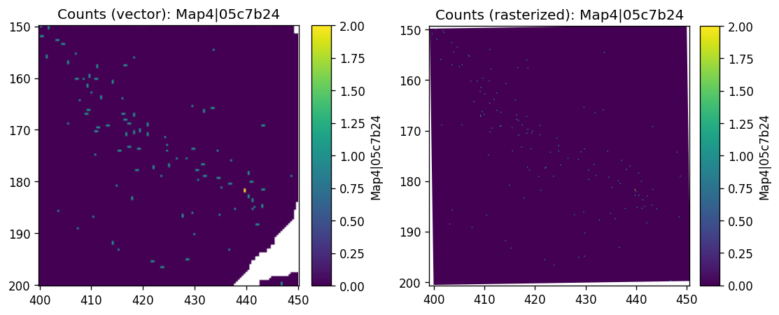
Or a zoomed-in view at a subregion (2µm resolution):

%%time
sdata_small = sdata.query.bounding_box(
    min_coordinate=[400, 150],
    max_coordinate=[450, 200],
    axes=("x", "y"),
    target_coordinate_system=f"{dataset_id}_downscaled_lowres",
)

axes = plt.subplots(1, 2, figsize=(10, 5))[1].flatten()
sdata_small.pl.render_shapes(f"{dataset_id}_square_002um", color=probe_name).pl.show(
    coordinate_systems=f"{dataset_id}_downscaled_lowres",
    ax=axes[0], title=f"Counts (vector): {probe_name}"
)
sdata_small.pl.render_images(f"rasterized_002um", channel=probe_name).pl.show(
    coordinate_systems=f"{dataset_id}_downscaled_lowres",
    ax=axes[1], title=f"Counts (rasterized): {probe_name}"
)
plt.subplots_adjust(wspace=0.5)
plt.show()

CPU times: user 3.52 s, sys: 429 ms, total: 3.95 s
Wall time: 3.97 s

Spatial variability testing with SplisosmFFT

To detect probe usage variation within a given gene, we run spatial variability test using hsic-ir.

Data filtering and model setup

Probe filtering criteria:

• min_counts: minimum total UMI count across all bins.

• min_bin_pct: minimum fraction of bins in which a probe must be detected.

• Genes with fewer than two passing probes are automatically excluded.

model = SplisosmFFT(
    neighbor_degree=1, # for rectangular bins, 1st degree = 4 nearest neighbors
    rho=0.99
)
model.setup_data(
    sdata=sdata,
    bins=test_bins_element,
    table_name=test_table,
    col_key="array_col",
    row_key="array_row",
    layer="counts",
    group_iso_by=group_iso_by,
    gene_names=gene_name_col, # 'gene_name'
    # optional probe filtering
    min_counts=min_counts,
    min_bin_pct=min_bin_pct,
    filter_single_iso_genes=True
)
model

=== SplisosmFFT
- Number of genes: 6224
- Number of spots: 98917
- Number of spots after rasterization: 124344
- Number of covariates: 0
- Average isoforms per gene: 2.7
=== Model configurations
- Neighborhood degree: 1
- Spatial autocorrelation rho: 0.99
=== Test results
- Spatial variability: NA
- Differential usage: NA

Extract gene-level summary statistics:

%%time
gene_meta = model.extract_feature_summary(level='gene')
gene_meta.sort_values('perplexity', ascending=False).head(5)

Genes: 100%|██████████| 6224/6224 [00:03<00:00, 1604.73it/s]

CPU times: user 4.05 s, sys: 314 ms, total: 4.36 s
Wall time: 4.41 s

	n_isos	perplexity	pct_bin_on	count_avg	count_std	major_ratio_avg
gene
Lrp1b	9	6.876322	0.204121	0.297128	0.723107	0.373754
Shank3	6	5.873075	0.228313	0.283612	0.582347	0.207386
Dusp3	6	5.868889	0.145162	0.171143	0.451044	0.223345
Auts2	6	5.863693	0.142402	0.176431	0.486012	0.222840
Mrtfb	6	5.777855	0.091410	0.104815	0.354134	0.235050

Probe-level summary is also available:

probe_meta = model.extract_feature_summary(level='isoform')
probe_meta.sort_values('gene_name', ascending=False).head(5)

	gene_ids	probe_ids	feature_types	filtered_probes	gene_name	genome	probe_region	pct_bin_on	count_total	count_avg	count_std	ratio_total	ratio_avg	ratio_std
Zzz3|e6db6c7	ENSMUSG00000039068	ENSMUSG00000039068|Zzz3|e6db6c7	Gene Expression	True	Zzz3	GRCm39	unspliced	0.010160	1021.0	0.010322	0.102658	0.313671	0.314407	0.460947
Zzz3|78e9dcb	ENSMUSG00000039068	ENSMUSG00000039068|Zzz3|78e9dcb	Gene Expression	True	Zzz3	GRCm39	unspliced	0.011302	1141.0	0.011535	0.108935	0.350538	0.350133	0.473619
Zzz3|208a79a	ENSMUSG00000039068	ENSMUSG00000039068|Zzz3|208a79a	Gene Expression	True	Zzz3	GRCm39	unspliced	0.010787	1093.0	0.011050	0.107114	0.335791	0.335460	0.469648
Zyx|7e650fc	ENSMUSG00000029860	ENSMUSG00000029860|Zyx|7e650fc	Gene Expression	True	Zyx	GRCm39	unspliced	0.013183	1339.0	0.013537	0.118664	0.504902	0.507246	0.495824
Zyx|680c694	ENSMUSG00000029860	ENSMUSG00000029860|Zyx|680c694	Gene Expression	True	Zyx	GRCm39	spliced	0.012819	1313.0	0.013274	0.118524	0.495098	0.492754	0.495824

Running spatial variability test

%%time

model.test_spatial_variability(
    method="hsic-ir",
    ratio_transformation="none",
    n_jobs=-1,
    print_progress=True,
)
sv_res_16um = model.get_formatted_test_results(
    "sv", with_gene_summary=True
).sort_values("pvalue_adj")

SV [hsic-ir]: 100%|██████████| 6224/6224 [01:39<00:00, 62.33it/s]

CPU times: user 3min 3s, sys: 30.3 s, total: 3min 34s
Wall time: 1min 40s

Top genes, sorted by adjusted p-value:

sig_001 = int((sv_res_16um["pvalue_adj"] < 0.01).sum())
print(
    "Spatially variably processed genes (FDR < 0.01, 16um): "
    f"{sig_001} out of {sv_res_16um.shape[0]} total genes"
)
sv_res_16um.head(5)

Spatially variably processed genes (FDR < 0.01, 16um): 196 out of 6226 total genes

	gene	statistic	pvalue	pvalue_adj	n_isos	perplexity	pct_bin_on	count_avg	count_std	major_ratio_avg
3964	Syt1	0.000003	0.000000e+00	0.000000e+00	3	2.628424	0.387153	0.758151	1.310308	0.584887
3517	Map4	0.000005	0.000000e+00	0.000000e+00	6	5.579242	0.347968	0.494172	0.839410	0.268749
1805	Gabbr1	0.000003	1.077128e-258	2.234681e-255	6	5.344769	0.283450	0.401003	0.768475	0.262467
1463	Oxr1	0.000002	1.293053e-135	2.011991e-132	5	4.394658	0.203888	0.274887	0.630308	0.306204
2276	Rabgap1l	0.000003	1.371692e-81	1.707482e-78	6	5.325925	0.242779	0.335079	0.701223	0.279439

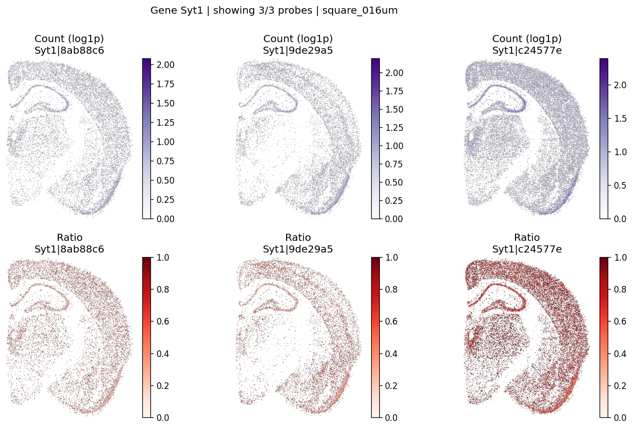
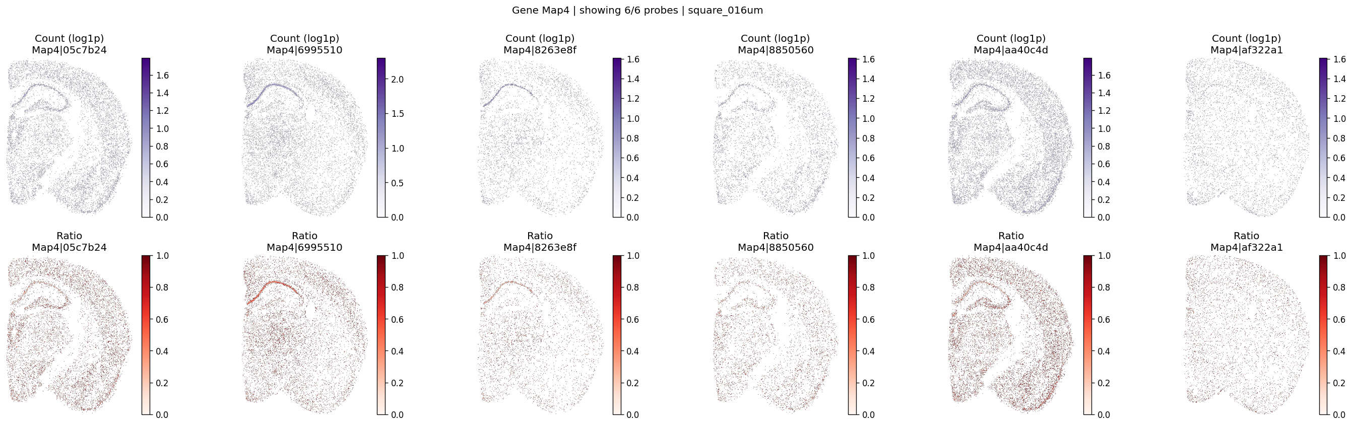
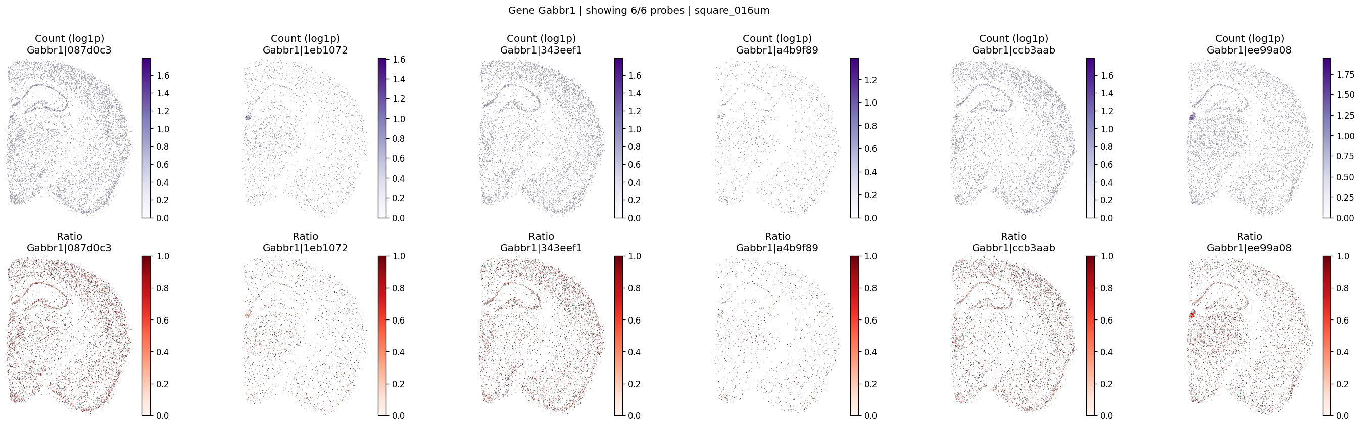
Visualize significant events

The helper below renders per-probe log1p counts and within-gene ratios on the testing grid.

def ensure_rasterized(sdata, bin_table: str, bin_element: str, layer: str = "counts"):
    raster_key = f"rasterized_{bin_table}_{layer}"
    if raster_key in sdata.images:
        return raster_key

    adata = sdata.tables[bin_table]
    adata.X = adata.layers[layer]
    if hasattr(adata.X, "tocsc") and getattr(adata.X, "format", None) != "csc":
        adata.X = adata.X.tocsc()

    sdata[raster_key] = rasterize_bins(
        sdata,
        bins=bin_element,
        table_name=bin_table,
        col_key="array_col",
        row_key="array_row",
    )
    return raster_key

The plotting function checks probe availability, lazily rasterizes data on demand, computes log1p counts and within-gene ratios, and optionally masks zero values.

def plot_gene_probe_maps(
    sdata,
    bin_table: str,
    bin_element: str,
    gene_id: str,
    probe_meta: pd.DataFrame | None = None,
    group_col: str = "gene_ids",
    max_probes: int = 4,
    hide_zero_count: bool = True,
    hide_zero_ratio: bool = True,
):
    adata = sdata.tables[bin_table]
    if probe_meta is None:
        probe_meta = adata.var.copy()

    if group_col not in probe_meta.columns:
        raise ValueError(f"'{group_col}' not found in probe_meta columns")

    probe_names = probe_meta.index[
        probe_meta[group_col].astype(str) == str(gene_id)
    ].tolist()
    if len(probe_names) == 0:
        raise ValueError(f"No probes found for gene id '{gene_id}'")
    if any(probe not in adata.var_names for probe in probe_names):
        raise ValueError(f"Some probes not found in {bin_table}.var_names")
    n_probes = len(probe_names)
    n_shown = min(n_probes, max_probes)
    probe_names = probe_names[:n_shown]

    raster_key = ensure_rasterized(sdata, bin_table=bin_table, bin_element=bin_element)
    data = sdata[raster_key].sel(c=probe_names).values
    counts_cube = np.moveaxis(np.asarray(data, dtype=float), 0, -1)

    counts_flat = counts_cube.reshape(-1, counts_cube.shape[-1])
    ratios_flat = counts_to_ratios(counts_flat, transformation="none", nan_filling="none")
    ratios_cube = ratios_flat.numpy().reshape(counts_cube.shape)

    n_probe = counts_cube.shape[-1]
    fig, axes = plt.subplots(2, n_probe, figsize=(4 * n_probe, 7), squeeze=False)

    for i, probe in enumerate(probe_names):
        c = counts_cube[:, :, i]
        r = ratios_cube[:, :, i]
        if hide_zero_count:
            c = np.where(c == 0, np.nan, c)
        if hide_zero_ratio:
            r = np.where(r == 0, np.nan, r)

        im0 = axes[0, i].imshow(np.log1p(c), cmap="Purples", vmin=0.0)
        axes[0, i].set_title(f"Count (log1p)\n{probe}")
        axes[0, i].axis("off")
        fig.colorbar(im0, ax=axes[0, i], fraction=0.046, pad=0.04)

        vmax = np.nanpercentile(ratios_cube, 99) if np.isfinite(ratios_cube).any() else 1.0
        im1 = axes[1, i].imshow(r, cmap="Reds", vmin=0.0, vmax=vmax)
        axes[1, i].set_title(f"Ratio\n{probe}")
        axes[1, i].axis("off")
        fig.colorbar(im1, ax=axes[1, i], fraction=0.046, pad=0.04)

    fig.suptitle(f"Gene {gene_id} | showing {n_shown}/{n_probes} probes | {bin_table}", y=1)
    fig.tight_layout()
    plt.show()

top_genes = sv_res_16um.head(10)["gene"].astype(str).tolist()
top_genes[:5]

['Syt1', 'Map4', 'Gabbr1', 'Oxr1', 'Rabgap1l']

for gene_id in top_genes[:3]:
    plot_gene_probe_maps(
        sdata=sdata,
        bin_table=test_table,
        bin_element=test_bins_element,
        gene_id=gene_id,
        group_col='gene_name',
        max_probes=6,
        probe_meta=probe_meta,
        hide_zero_ratio=True,
    )

%%time
# Example: inspect a specific gene manually
plot_gene_probe_maps(
    sdata, test_table, test_bins_element, 
    gene_id="Gnas", 
    group_col='gene_name', 
    probe_meta=probe_meta
)

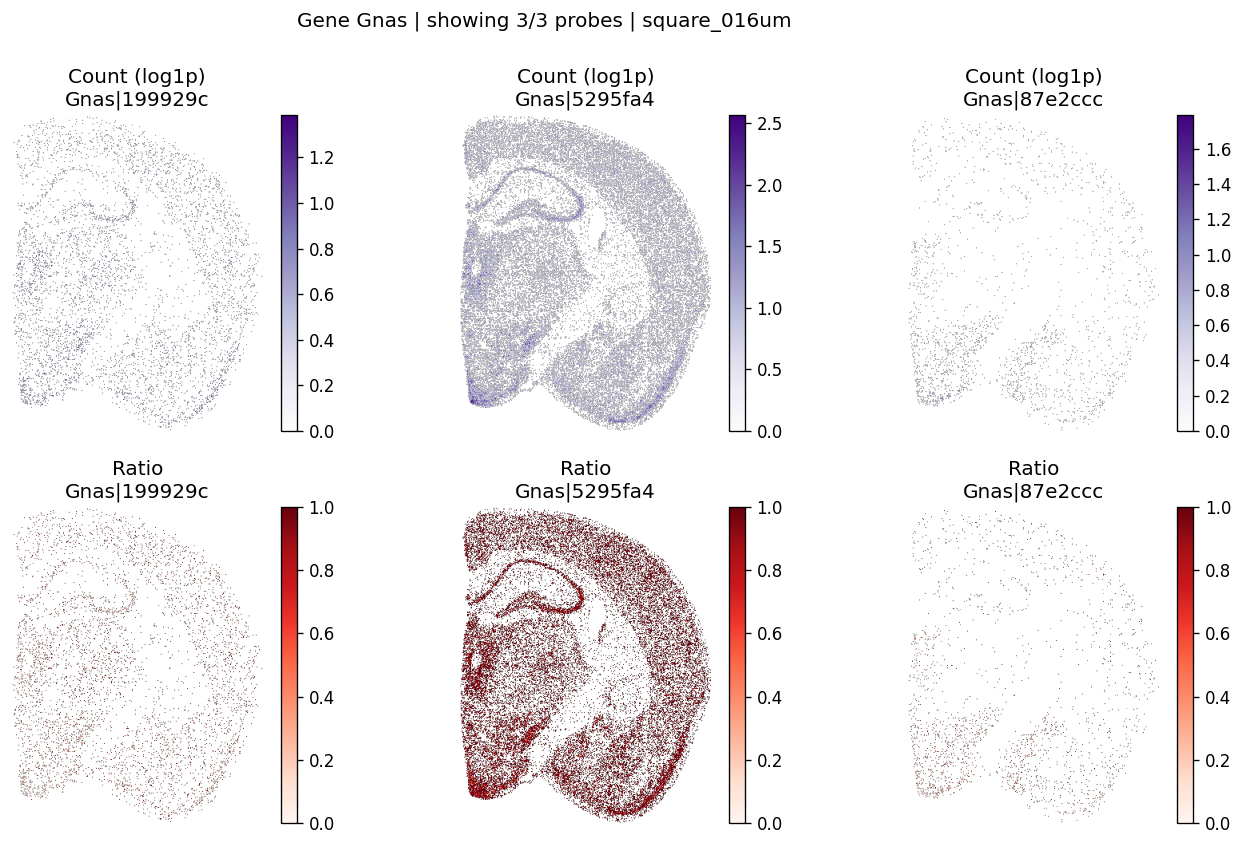
CPU times: user 225 ms, sys: 21.9 ms, total: 246 ms
Wall time: 247 ms

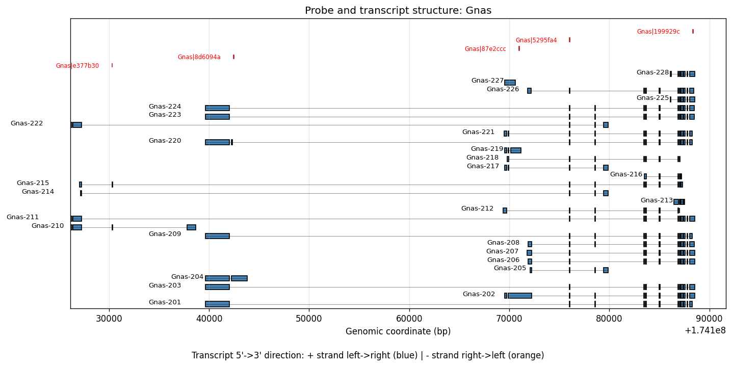
To see the spatially variable transcript regions, we can visualize the 10x reference probe sets along with a matched transcript reference. The following files need to be downloaded and provided as input:

• Visium_Mouse_Transcriptome_Probe_Set_v2.1.0_GRCm39-2024-A.bed from 10x Genomics

• gencode.vM33.annotation.gtf.gz from GENCODE

Show code cell source

Hide code cell source

def plot_probe_transcript_structure(
    gene_name: str,
    bed_file: str | Path,
    gtf_file: str | Path,
    figsize: tuple[float, float] = (12, 6),
):
    """Visualize probe and transcript exon structure for a given gene.

    Reads probe coordinates from a BED12 file and transcript structure from a GTF file,
    then plots them on the same genomic coordinate axis. Each probe is shown on its
    own row to avoid overlap, and transcripts are labeled by transcript_name.
    """
    import gzip

    bed_file = Path(bed_file)
    gtf_file = Path(gtf_file)

    # Read BED12 file and keep block model columns.
    bed_cols = [
        "chrom", "start", "end", "name", "score", "strand",
        "thickStart", "thickEnd", "itemRgb", "blockCount", "blockSizes", "blockStarts",
    ]
    bed_df = pd.read_csv(
        bed_file,
        sep="\t",
        header=None,
        names=bed_cols,
        usecols=list(range(12)),
    )

    # Filter probes by gene name using pipe-delimited match (format: gene_id|gene_name|hash).
    probe_mask = bed_df["name"].astype(str).str.contains(rf"\|{gene_name}\|", case=False, na=False)
    probes = bed_df[probe_mask].copy()

    if probes.empty:
        warnings.warn(f"No probes found for gene '{gene_name}' in {bed_file}")

    # Extract shorter probe labels for common formats.
    def shorten_probe_id(full_name: str) -> str:
        text = str(full_name)
        if "|" in text:
            parts = text.split("|")
            if len(parts) >= 2:
                return "|".join(parts[1:])
        return text

    probes["probe_id"] = probes["name"].apply(shorten_probe_id)

    # Convert BED12 blocks to absolute genomic coordinates per probe.
    def parse_blocks(row: pd.Series) -> list[tuple[int, int]]:
        starts = [int(x) for x in str(row["blockStarts"]).strip(",").split(",") if x != ""]
        sizes = [int(x) for x in str(row["blockSizes"]).strip(",").split(",") if x != ""]
        n = min(int(row["blockCount"]), len(starts), len(sizes))
        blocks = []
        for i in range(n):
            block_start = int(row["start"]) + starts[i]
            block_end = block_start + sizes[i]
            blocks.append((block_start, block_end))
        return blocks

    if not probes.empty:
        probes["blocks"] = probes.apply(parse_blocks, axis=1)

    # Read GTF and filter transcripts by gene name
    if str(gtf_file).endswith(".gz"):
        gtf_opener = lambda f: gzip.open(f, "rt")
    else:
        gtf_opener = open

    transcripts_by_id = {}
    with gtf_opener(gtf_file) as f:
        for line in f:
            if line.startswith("#"):
                continue
            fields = line.rstrip("\n").split("\t")
            if len(fields) < 9:
                continue
            ftype, start, end = fields[2], int(fields[3]), int(fields[4])
            attrs = {}
            for attr in fields[8].split("; "):
                if " " in attr:
                    k, v = attr.split(" ", 1)
                    attrs[k] = v.strip('"')

            # Match gene by gene_name or gene_id
            if attrs.get("gene_name", "").lower() != gene_name.lower() and \
               attrs.get("gene_id", "").lower() != gene_name.lower():
                continue

            tx_id = attrs.get("transcript_id", "unknown")
            if tx_id not in transcripts_by_id:
                tx_name = attrs.get("transcript_name", tx_id)
                transcripts_by_id[tx_id] = {
                    "chrom": fields[0],
                    "strand": fields[6],
                    "tx_name": tx_name,
                    "exons": [],
                }

            if ftype == "exon":
                transcripts_by_id[tx_id]["exons"].append((start, end))

    # Create plot
    fig, ax = plt.subplots(figsize=figsize)

    # Plot transcripts first
    y_pos = 0
    x_mins = []
    x_maxs = []

    # Strand color coding for cleaner direction cues.
    strand_colors = {
        "+": "steelblue",
        "-": "darkorange",
    }

    if transcripts_by_id:
        for tx_id, tx_info in sorted(transcripts_by_id.items()):
            exons = sorted(tx_info["exons"])
            if not exons:
                continue

            # Draw introns (thin line)
            min_coord = min(e[0] for e in exons)
            max_coord = max(e[1] for e in exons)
            x_mins.append(min_coord)
            x_maxs.append(max_coord)
            ax.plot([min_coord, max_coord], [y_pos, y_pos], "k-", linewidth=0.5, alpha=0.5)

            # Draw exons (thick boxes), color by strand
            strand = str(tx_info.get("strand", "."))
            tx_color = strand_colors.get(strand, "gray")
            for start, end in exons:
                ax.barh(y_pos, end - start, left=start, height=0.6, color=tx_color, edgecolor="black")

            # Label with transcript_name
            tx_name = tx_info.get("tx_name", tx_id[:20])
            ax.text(min_coord - (max_coord - min_coord) * 0.05, y_pos, tx_name[:30], ha="right", fontsize=8)
            y_pos += 1

    # Plot probes, each on its own row, using BED12 block segments.
    probe_rows = probes.sort_values(["chrom", "start", "end"]) if not probes.empty else probes

    for idx, (_, row) in enumerate(probe_rows.iterrows()):
        probe_y = y_pos + idx
        blocks = row["blocks"] if isinstance(row["blocks"], list) and row["blocks"] else [(int(row["start"]), int(row["end"]))]
        probe_min = min(b[0] for b in blocks)
        probe_max = max(b[1] for b in blocks)
        x_mins.append(probe_min)
        x_maxs.append(probe_max)

        ax.plot([probe_min, probe_max], [probe_y, probe_y], color="firebrick", linewidth=0.7, alpha=0.6)
        for block_start, block_end in blocks:
            ax.barh(
                probe_y,
                block_end - block_start,
                left=block_start,
                height=0.45,
                color="salmon",
                edgecolor="firebrick",
            )

    x_pad = max(1.0, (max(x_maxs) - min(x_mins)) * 0.02) if x_mins and x_maxs else 1.0

    for idx, (_, row) in enumerate(probe_rows.iterrows()):
        probe_y = y_pos + idx
        blocks = row["blocks"] if isinstance(row["blocks"], list) and row["blocks"] else [(int(row["start"]), int(row["end"]))]
        probe_min = min(b[0] for b in blocks)
        ax.text(probe_min - x_pad, probe_y, row["probe_id"], ha="right", va="center", fontsize=7, color="red")

    y_pos += len(probe_rows)

    # Format axes
    ax.set_ylim(-0.5, y_pos + 0.5)
    ax.set_xlabel("Genomic coordinate (bp)")
    ax.set_ylabel("")
    ax.set_yticks([])
    ax.set_title(f"Probe and transcript structure: {gene_name}")
    ax.grid(True, axis="x", alpha=0.3)

    # Place strand direction note as a single centered row below the plot.
    direction_note = "Transcript 5'->3' direction: + strand left->right (blue) | - strand right->left (orange)"
    fig.text(0.5, 0.01, direction_note, ha="center", va="bottom", fontsize=10, color="black")

    # Reserve bottom margin for the legend row.
    fig.tight_layout(rect=(0.0, 0.05, 1.0, 1.0))
    plt.show()

%%time
plot_probe_transcript_structure(
    gene_name="Gnas",
    bed_file=visium_hd_outs / "Visium_Mouse_Transcriptome_Probe_Set_v2.1.0_GRCm39-2024-A.bed",
    gtf_file=reference_path / "gencode.vM33.annotation.gtf.gz",
)

CPU times: user 6.33 s, sys: 64.3 ms, total: 6.39 s
Wall time: 6.45 s

Advanced analyses

Hyperparameter sensitivity check

A lightweight robustness check compares p-values under nearby kernel settings (neighbor_degree, rho).

# reusable setup parameters for multiple resolutions
setup_params = {
    'sdata': sdata,
    'bins': test_bins_element,
    'table_name': test_table,
    'col_key': "array_col",
    'row_key': "array_row",
    'layer': "counts",
    'group_iso_by': group_iso_by,
    'gene_names': gene_name_col,
    'min_counts': 100,
    'min_bin_pct': 0.05,
    'filter_single_iso_genes': True
}

Spectral analysis of kernel matrices

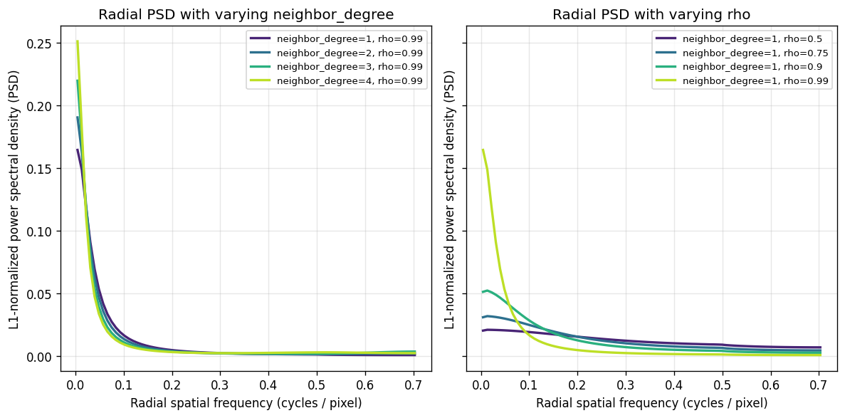
Two hyperparameters control the kernel: neighbor_degree (spatial graph connectivity; larger values capture more global structure) and rho (spectral decay; values closer to 1 concentrate energy on low-frequency patterns). The plots below show the normalized power spectral density under different settings.

%%time
def extract_l1_normalized_psd(model, bins=80):
    """Return radial PSD with L1 normalization for comparison across kernels."""
    freq_bins, psd = model.sp_kernel.power_spectral_density_1d(bins=bins)
    # scale eigenvalues to sum-one
    denom = float(np.sum(np.abs(psd)))
    if denom <= 0.0:
        raise ValueError("Power spectral density has zero total magnitude.")
    return freq_bins, psd / denom


def plot_psd_family(configs, title, ax, bins=80):
    colors = plt.cm.viridis(np.linspace(0.1, 0.9, len(configs)))

    for cfg, color in zip(configs, colors):
        m = SplisosmFFT(**cfg)
        m.setup_data(**setup_params)
        freq_bins, psd_l1 = extract_l1_normalized_psd(m, bins=bins)
        label = ", ".join([f"{key}={value}" for key, value in cfg.items()])
        ax.plot(freq_bins, psd_l1, color=color, linewidth=2.0, label=label)

    ax.set_xlabel("Radial spatial frequency (cycles / pixel)")
    ax.set_ylabel("L1-normalized power spectral density (PSD)")
    ax.set_title(title)
    ax.grid(True, alpha=0.3)
    ax.legend(fontsize=8)


neighbor_configs = [
    {"neighbor_degree": 1, "rho": 0.99},
    {"neighbor_degree": 2, "rho": 0.99},
    {"neighbor_degree": 3, "rho": 0.99},
    {"neighbor_degree": 4, "rho": 0.99},
]

rho_configs = [
    {"neighbor_degree": 1, "rho": 0.50},
    {"neighbor_degree": 1, "rho": 0.75},
    {"neighbor_degree": 1, "rho": 0.90},
    {"neighbor_degree": 1, "rho": 0.99},
]

fig, axes = plt.subplots(1, 2, figsize=(10, 5), sharey=True)
plot_psd_family(
    neighbor_configs,
    title="Radial PSD with varying neighbor_degree",
    ax=axes[0],
    bins=80,
)
plot_psd_family(
    rho_configs,
    title="Radial PSD with varying rho",
    ax=axes[1],
    bins=80,
)
plt.tight_layout()
plt.show()

CPU times: user 23.2 s, sys: 1.06 s, total: 24.2 s
Wall time: 24.2 s

rho is the more effective parameter for emphasizing low-frequency spatial patterns.

Effect on spatial variability results

Compare gene rankings across hyperparameter settings:

%%time
configs = [
    {"neighbor_degree": 1, "rho": 0.99},
    {"neighbor_degree": 2, "rho": 0.99},
    {"neighbor_degree": 1, "rho": 0.90},
]

cfg_results = []
for cfg in configs:
    m = SplisosmFFT(neighbor_degree=cfg["neighbor_degree"], rho=cfg["rho"])
    m.setup_data(**setup_params)
    m.test_spatial_variability(
        method='hsic-ir',
        ratio_transformation='none',
        n_jobs=-1,
        print_progress=True,
    )
    res = m.get_formatted_test_results("sv")[["gene", "pvalue", "pvalue_adj"]].copy()
    tag = f"k{cfg['neighbor_degree']}_rho{cfg['rho']}"
    res = res.rename(columns={"pvalue": f"p_{tag}", "pvalue_adj": f"padj_{tag}"})
    cfg_results.append(res)

SV [hsic-ir]: 100%|██████████| 1065/1065 [00:16<00:00, 66.37it/s]
SV [hsic-ir]: 100%|██████████| 1065/1065 [00:16<00:00, 65.08it/s]
SV [hsic-ir]: 100%|██████████| 1065/1065 [00:16<00:00, 63.78it/s]

CPU times: user 1min 38s, sys: 14.7 s, total: 1min 53s
Wall time: 59 s

merged = cfg_results[0]
for res in cfg_results[1:]:
    merged = merged.merge(res, on="gene", how="inner")

p_cols = [c for c in merged.columns if c.startswith("p_")]
print("Spearman correlation across hyperparameter settings:")
display(merged[p_cols].corr(method="spearman"))

Spearman correlation across hyperparameter settings:

	p_k1_rho0.99	p_k2_rho0.99	p_k1_rho0.9
p_k1_rho0.99	1.000000	0.992542	0.818208
p_k2_rho0.99	0.992542	1.000000	0.757281
p_k1_rho0.9	0.818208	0.757281	1.000000

pairs = list(combinations(p_cols, 2))
if pairs:
    fig, axes = plt.subplots(1, len(pairs), figsize=(3 * len(pairs), 3), squeeze=False)
    axes = axes.ravel()

    for ax, (x_col, y_col) in zip(axes, pairs):
        x = merged[x_col].to_numpy()
        y = merged[y_col].to_numpy()
        corr, pval = spearmanr(x, y)

        ax.scatter(x + 1e-100, y + 1e-100, s=8, alpha=0.5)
        ax.set_xscale("log")
        ax.set_yscale("log")
        ax.set_xlabel(x_col)
        ax.set_ylabel(y_col)
        ax.set_title(f"Spearman ρ={corr:.3f}")
        ax.grid(True, alpha=0.3)

        low = 1e-100
        high = max(np.max(x), np.max(y))
        ax.plot([low, high], [low, high], "r--", alpha=0.5, linewidth=1.5)
        ax.set_xlim(low, high)
        ax.set_ylim(low, high)

    plt.tight_layout()
    plt.show()

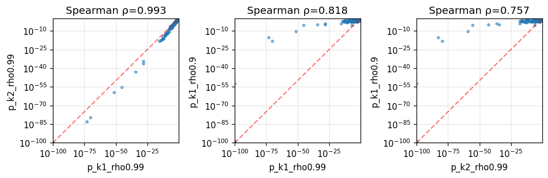
Gene rankings are more sensitive to rho than neighbor_degree. For this mouse brain dataset, most spatial patterns are low-frequency, so decreasing rho reduces statistical power.

Spatial resolution comparison

For illustration, we use the top 200 genes from the 16µm analysis as the reference set:

# np.random.seed(42)
# gene_names = sdata.tables[test_table].var['gene_name'].unique()
# gene_subset = np.random.choice(gene_names, size=200, replace=False)
gene_subset = sv_res_16um.sort_values('pvalue').head(200)['gene'].astype(str).tolist()

Run spatial variability tests across all three resolutions:

%%time
# Compare results across 2µm, 8µm, 16µm resolutions
resolutions = [
    {'bin': f'{dataset_id}_square_002um', 'table_name': 'square_002um'},
    {'bin': f'{dataset_id}_square_008um', 'table_name': 'square_008um'},
    {'bin': f'{dataset_id}_square_016um', 'table_name': 'square_016um'},
]

res_results = []
for res in resolutions:
    m = SplisosmFFT(neighbor_degree=1, rho=0.99)
    sdata_subset = sd.filter_by_table_query(
        sdata,
        table_name=res['table_name'],
        var_expr=an.col('gene_name').is_in(gene_subset),
    )
    m.setup_data(
        sdata_subset,
        bins=res['bin'],
        table_name=res['table_name'],
        col_key="array_col",
        row_key="array_row",
        layer="counts",
        group_iso_by="gene_ids",
        gene_names="gene_name",
        min_counts=10,
        min_bin_pct=0.0
    )
    m.test_spatial_variability(method='hsic-ir')
    results = m.get_formatted_test_results('sv')[['gene', 'pvalue']].copy()
    results.rename(columns={'pvalue': f"p_{res['table_name']}"}, inplace=True)
    res_results.append(results)

SV [hsic-ir]: 100%|██████████| 200/200 [02:30<00:00,  1.33it/s]
SV [hsic-ir]: 100%|██████████| 200/200 [00:04<00:00, 47.29it/s]
SV [hsic-ir]: 100%|██████████| 200/200 [00:01<00:00, 143.82it/s]

CPU times: user 6min 48s, sys: 7min, total: 13min 48s
Wall time: 2min 56s

merged = res_results[0]
for res in res_results[1:]:
    merged = merged.merge(res, on="gene", how="inner")

p_cols = [c for c in merged.columns if c.startswith("p_")]
print("Spearman correlation across spatial resolutions:")
display(merged[p_cols].corr(method="spearman"))

Spearman correlation across spatial resolutions:

	p_square_002um	p_square_008um	p_square_016um
p_square_002um	1.000000	0.607920	0.510704
p_square_008um	0.607920	1.000000	0.705029
p_square_016um	0.510704	0.705029	1.000000

pairs = list(combinations(p_cols, 2))
if pairs:
    fig, axes = plt.subplots(1, len(pairs), figsize=(3 * len(pairs), 3), squeeze=False)
    axes = axes.ravel()

    for ax, (x_col, y_col) in zip(axes, pairs):
        x = merged[x_col].to_numpy()
        y = merged[y_col].to_numpy()
        corr, pval = spearmanr(x, y)

        ax.scatter(x + 1e-150, y + 1e-150, s=8, alpha=0.5)
        ax.set_xscale("log")
        ax.set_yscale("log")
        ax.set_xlabel(x_col)
        ax.set_ylabel(y_col)
        ax.set_title(f"Spearman ρ={corr:.3f}")
        ax.grid(True, alpha=0.3)

        low = 1e-150
        high = max(np.max(x), np.max(y))
        ax.plot([low, high], [low, high], "r--", alpha=0.5, linewidth=1.5)
        ax.set_xlim(low, high)
        ax.set_ylim(low, high)

    plt.tight_layout()
    plt.show()

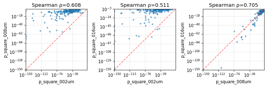
Gene rankings are broadly consistent across resolutions, especially between 16µm and 8µm. The 2µm analysis shows stronger statistical significance, likely because the kernel places more weight on low-frequency patterns at finer scales.

Method comparison: SplisosmFFT vs SplisosmNP

Compare FFT-accelerated and non-parametric spatial variability tests at 16 µm resolution.

The eigenvalue null (null_method="eig") supports a low-rank approximation via null_configs={"approx_rank": k}. A higher rank gives more accurate p-values at increased cost. Here we use approx_rank=20 for a fast demonstration.

%%time
# Run SplisosmNP at 16µm for direct comparison with SplisosmFFT
model_np = SplisosmNP(
    k_neighbors=4,
    rho=0.99,
    standardize_cov=False, # faster
)
model_np.setup_data(
    adata=sdata.tables[test_table],
    spatial_key='spatial', # adata.obsm key for spatial coordinates
    layer='counts',
    group_iso_by=group_iso_by, # 'gene_ids'
    gene_names=gene_name_col, # 'gene_name'
    min_counts=min_counts,
    min_bin_pct=min_bin_pct,
    filter_single_iso_genes=True,
    min_component_size=10 # remove disconnected tissue fragments if any
)

CPU times: user 1.37 s, sys: 318 ms, total: 1.69 s
Wall time: 1.98 s

%%time
model_np.test_spatial_variability(
    method='hsic-ir',
    null_configs={"approx_rank": 20},
    ratio_transformation='none',
    print_progress=True,
)

SV [hsic-ir]: 100%|██████████| 6224/6224 [00:08<00:00, 732.86it/s]

CPU times: user 52.9 s, sys: 21.6 s, total: 1min 14s
Wall time: 11.2 s

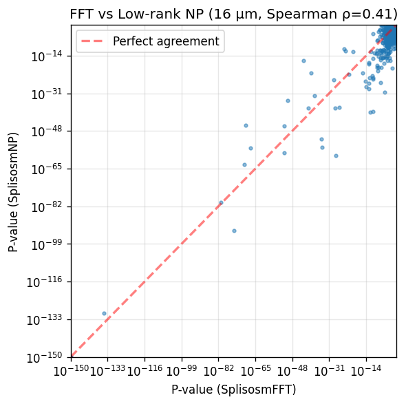
Compare p-values between SplisosmFFT and SplisosmNP:

# Extract results and merge
sv_np = model_np.get_formatted_test_results('sv')[['gene', 'pvalue']].copy()
sv_np = sv_np.rename(columns={'pvalue': 'pvalue_np'})

comparison = sv_res_16um[['gene', 'pvalue']].copy()
comparison = comparison.rename(columns={'pvalue': 'pvalue_fft'})
comparison = comparison.merge(sv_np, on='gene', how='inner')

corr, _ = spearmanr(comparison['pvalue_fft'], comparison['pvalue_np'])

print(f'Genes tested in both methods: {len(comparison)}')
print(f'== Significant in SplisosmFFT (FDR < 0.01): {(comparison["pvalue_fft"] < 0.01).sum()}')
print(f'== Significant in SplisosmNP (FDR < 0.01): {(comparison["pvalue_np"] < 0.01).sum()}')
print(f'== P-value correlation (Spearman rho): {corr:.4f}')

Genes tested in both methods: 6230
== Significant in SplisosmFFT (FDR < 0.01): 654
== Significant in SplisosmNP (FDR < 0.01): 1075
== P-value correlation (Spearman rho): 0.4134

# Scatter plot comparison
fig, ax = plt.subplots(figsize=(5, 5))
x = comparison['pvalue_fft'].to_numpy()
y = comparison['pvalue_np'].to_numpy()

ax.scatter(x + 1e-150, y + 1e-150, s=8, alpha=0.5)
ax.set_xscale('log')
ax.set_yscale('log')
ax.set_xlabel('P-value (SplisosmFFT)')
ax.set_ylabel('P-value (SplisosmNP)')
ax.set_title(f'FFT vs Low-rank NP (16 µm, Spearman ρ={corr:.2f})')
ax.grid(True, alpha=0.3)

# Add diagonal reference line
lims = [1e-150, 1.0]
ax.plot(lims, lims, 'r--', alpha=0.5, label='Perfect agreement', linewidth=2)
ax.legend()
ax.set_xlim(lims)
ax.set_ylim(lims)

plt.tight_layout()
plt.show()

Summary and recommendations

Key findings:

1. Kernel spectra concentrate energy at low frequencies. Both neighbor_degree and rho shape the spectrum, but rho has the larger effect on downstream gene rankings. Kernels emphasizing low-frequency patterns tend to yield higher statistical power.

2. Spatial resolution trade-offs:

   • 16 µm: Fast and reliable — recommended for initial exploration.

   • 8 µm: High agreement with 16 µm results.

   • 2 µm: Highest resolution but slower and sparser.

3. Method equivalence: SplisosmFFT and SplisosmNP yield concordant rankings on regular grids, particularly for genes with strong spatial patterns.

Recommendations:

• Start with 16 µm binning for exploratory analysis.

• Refine with 8 µm if finer spatial detail is needed.

• Use SplisosmFFT on regular grids (Visium HD, Xenium binned data) with neighbor_degree=1, rho=0.99 as a robust default.

• Use SplisosmNP for irregular geometries (e.g., cell-segmented data).

For reproducibility

import sys
from datetime import date
import splisosm

print("Last updated:", date.today())
print("Python:", sys.version.split()[0])
print("splisosm:", getattr(splisosm, "__version__", "unknown"))

Last updated: 2026-04-20
Python: 3.12.13
splisosm: 1.1.1